Comeau, L.A. and S.E. Campana. 2003. Modifying thyroidal status in Atlantic cod by osmotic pump delivery of thryoid and antithyroid agents. Trans. Am. Fish. Soc. 132:1021-1026.
Secor, D.H., J.M. Dean and S.E. Campana. 1995. Introduction. Fish otoliths: faithful biological and environmental chronometers? P. xxv-xxvii. In: D.H. Secor, J. M. Dean and S.E. Campana [ed]. Recent Developments in Fish Otolith Research. Univ. of South Carolina Press. Columbia, S.C.
Campana, S. E. 1987. Comparison of two length‑based indices of abundance in adjacent haddock stocks (Melanogrammus aeglefinus) on the Scotian Shelf. J. Cons. Int. Explor. Mer 44:43‑55.
Microsampling techniques are utilized to mechanically extract a portion of the otolith for subsequent analysis. Portions can be extracted as either powders, milled from discrete depths (e.g. annual growth zones) or as cores (e.g. first year of growth).
Assays for bomb radiocarbon and stable isotope ratios are examples of applications where a particular age or date range in the otolith is required. For these applications the best sampling procedures involve microsampling or coring techniques which physically remove a discrete portion of the otolith.
1) Microsampling Device (automated):
We have prepared a 15-minute VIDEO DEMONSTRATION of the use of the Micromill for isolating otolith material, which provides an easy and complete introduction to the process. The information below also describes micromilling, but provides more detail on some of the materials and suppliers than does the video.
A photograph of our Micromill microsampling device is depicted below. This system includes the following:
Micromill microsampling device
Pentium-based PC installed with MicroMill software, Coreco Bandit video board and drivers.
17" monitor, maximum resolution of 1280x1024.
MicroMill sampler (New Wave Research) consists of a Leica stereo microscope fitted with a high resolution colour video camera, fine resolution (0.25 micron) motorized XYZ stages, high torque milling chuck with adjustable speed and carbide tipped or hardened cobalt steel milling bits.
Using on screen digitization of the sample area and precise depth control this system permits automated and accurate microsampling.
Close up of the Micromill drill bit and an otolith cross section.
In our usual mode of operation the drill bit is used to carve out areas of the otolith, leaving discrete chunks which can be decontaminated prior to analysis.
2) Hand-held Drill:
Hand-held microsampler
A photograph of our hand-held sampling setup is depicted to the right. This system includes the following:
a selection of drilling bits including diamond-tipped orb and circular cutting tools
Wild stereo microscope
High-intensity fiber optic illuminator (Nikon) with dual gooseneck cables
Acrylic containment device, to prevent loss of sample
HEPA filter vacuuming unit to remove fine dust from the work area
Using a combination of drilling and sculpturing techniques this hand-held setup offers an affordable alternative to the automated MicroMill system. Although accessible, this system is labour intensive to operate and its affordability is outweighed by its lack of precision.
Information from this page should be cited as: Campana, S.E., and C. M. Jones. 1992. Analysis of otolith microstructure data, p. 73-100. In D. K. Stevenson and S. E. Campana [ed.] Otolith microstructure examination and analysis. Can. Spec. Publ. Fish. Aquat. Sci. 117.
The preparation and interpretation of an otolith is only the first step in the extraction of useful information about a fish. It is understandable that the technical difficulties associated with otolith microstructure examination can occupy much of a researcher's time. However, the analysis of the resulting data is often given so little attention that much of the information acquired so painstakingly is effectively lost. Indeed, many publications reporting otolith data contain only the size-at-age data, perhaps in the form of a scatterplot, thus ignoring what is often more interesting and useful information. Of course, most analyses, even those as simple as growth rate calculations, require complete and representative sampling of all of the relevant cohorts/life history stages (see Butler, this volume). The intent of this chapter is to highlight the most useful and powerful applications of otolith microstructure examination, and in so doing, attempt to encourage a more complete analysis of otolith based data on a routine basis. Many of the analyses are not particularly difficult to undertake, but merely require some forethought as to the best way to proceed. Thus we shall also offer our views on the most appropriate way to approach and complete each analysis. Examples are given wherever possible.
Many of the applications which make use of otolith microstructure examination have analogs in other areas of fisheries science. Obvious examples include the estimation of age and growth rate, both of which have long been studied at the yearly level. However, a typical sequence of daily growth increments lends itself to most applications much better than those at the yearly level, largely because of the longer and temporally more exact sequence of marks in each otolith. In addition, applications such as hatch date analysis are almost unique to otolith microstructure studies. In this chapter, we shall review all of the major applications of otolith microstructure data, but focus our discussion on the analyses not generally found in other fields of research. The simulations and discussion of hatch date analysis are new, reflecting the still-evolving nature of this type of analysis. However, much of the remaining information has been presented elsewhere; this chapter simply serves to bring it all together in a coherent form, much of it for the first time.
Age Estimation
Conversion of Increment Counts to Age Estimates
Given a life history stage in a species in which daily increment formation has been validated (see Geffen, this volume), the number of daily increments must be proportional to, but not necessarily equal to, the age of the fish. Since the inner-most increment does not necessarily form at hatch, experimentation or observation is required to determine the age at which the first increment is formed. Of course, increment counts can be initiated at any otolith landmark to which an age can be reliably and consistently assigned; neither the inner-most increment nor the hatch check need be used. One example of an alternate landmark is that of a check formed at mouth-opening (Lagardère and Chaumillon 1988). Irrespective of the landmark used, age is then calculated as the sum of the age at landmark formation and increment count distal to that landmark. While fish age is the usual objective of otolith microstructure examination, individual increments can also be interpreted in terms of date of formation, through knowledge of the date of sampling (=date of formation of the marginal, or last-formed, increment). Dated increments are proving to be of increasing value to analyses cross-correlating environmental factors to the otolith growth sequence (e.g., Methot 1981; Campana and Hurley 1989; Suthers et al. 1989).
The estimation of age from daily increment counts is simple in principle, but the practice is confounded by the errors and uncertainties associated with microstructural examinations (see Neilson, this volume, and Campana, this volume). To some extent, the ageing uncertainties can be reduced through examination of multiple otoliths. All teleosts have three pairs of otoliths, of which two pairs are often interpretable. Since increment counting error is at least partially due to preparation artifacts, examination of both otoliths from a given pair can aid in reducing the variance (increasing the precision) of each age estimate. Where it can be demonstrated that other otolith types contain the same age information (or can be calibrated to the same age), more than one otolith pair can be read to further increase precision (Campana and Hurley 1989). Of course, peculiarities in the otolith microstructure attributable to fish growth will be reflected in all of the otoliths, and that source of error is unlikely to be reduced by multiple readings. It should also be noted that readings of multiple otoliths from a single fish are not equivalent to the same number of readings from a single otolith; the latter will reduce the variance attributable to counting error while the former will reduce the variance due to both counting and preparation error.
A single best estimate of age from a given fish will result from multiple readings of each of several otoliths, at least where possible. However, an overall average of all of the readings will seldom be appropriate. A more appropriate age estimation procedure involves: (1) the determination of the single "best" estimate of increment count for each otolith, (2) pooling of the increment counts from a given otolith type, (3) converting increment counts from each otolith type to age estimates, and (4) pooling the results from the otolith types. At least, this is the most appropriate procedure in theory. In practise, the time and effort involved in reading multiple otoliths from a single fish must be balanced against the benefits of increasing the number of fish which are examined. As a general rule of thumb, the examination of two otoliths (usually of a single otolith type) from each fish appears to be a useful compromise between within fish precision and overall sample size.
The single "best" estimate of increment count from a given otolith may be the mean of multiple counts if all counts were considered equally reliable. Use of a median, rather than a mean, reduces the influence of single, aberrant counts. However, since otolith readers often give higher credence to certain readings, some form of weighting in terms of reliability is often preferred. Weighting can be as described below, or can be slightly more subjective through selection of the single count with which the most confidence is associated. In most cases, the difference between the two weighting procedures will be minimal. After assigning a single increment count to each otolith, a single value is calculated for each otolith type, either by averaging or through weighted averaging. Increment counts from each otolith type are then converted to age estimates using the appropriate conversion (e.g., age = lapillar count + 2). The final stage is the averaging (weighted or unweighted) across otolith types. The mathematical algorithm for the single best increment count (Ctj) from the jth (first or second) otolith of the tth otolith type (eg. sagitta, lapillus, or asteriscus) is:
(1) Ctj=(∑1RXi⨯Wi)∑1RWi
where R represents the number of times that the otolith was counted, and Wi is the weight given to each count (Xi). Although statistical weights are often calculated as the inverse of the variance, there is no variance associated with a single count. A more useful approach here is to weight on the basis of perceived confidence in the otolith reading; an arbitrary scale from 1 (little confidence) to 5 (unambiguous count) for each otolith is one such approach. Calculation of the mean increment count for a given otolith type is a simple variant of Equation (1), whereby weights are either assigned to each otolith based on confidence, or the weights are assumed to be equal, resulting in a simple mean. After converting each of the otolith type increment counts to age estimates, the final (weighted) mean is then calculated across otolith types. It is important to note that the above procedure, whereby (weighted) means are calculated at each stage, is not equivalent to a (weighted) mean of all of the readings combined. As for the use of weighted means, weighting appears to be most important in the first two stages (calculation of the best increment count for each otolith and otolith type); unless one otolith type is clearly superior to the other, a simple mean across otolith types is probably sufficient.
Consider the following example, based on three readings each of two sagittae and one lapillus (one lapillus was lost during preparation). Confidence ranks were assigned on a scale of 1 (low confidence) to 5 (high confidence). Assume that increment counts were initiated at a check which formed one day after hatch:
Count
Rank
Count
Rank
Count
Rank
Weighted mean
Sag 1
20
5
18
4
28
1
20.0
Sag 2
22
4
23
3
19
4
21.2
Lap 1
19
4
20
4
21
4
20.0
Assuming that Sag I and Sag 2 were comparable in ease of interpretation, the mean Sag count would be 20.6. Converting the Sag and the Lap counts to ages (count + 1), and taking the mean, results in an age estimate of 21.3 d. Note the difference between this estimate and the simple mean of all of the above readings (=21.1 + 1 = 22.1 d). Note also that the otolith types were equally weighted in the calculation of the final age estimate, despite the fact that there were two sagittae and only one lapillus. Equal weighting is appropriate if the two otolith types differ in their ease of preparation and/or interpretation, yet there is no basis for considering one otolith type more reliable than the other. Where one otolith type is considered to be more reliable than the other, it is probably best to age only the reliable pair.
Accuracy and Precision
Age estimates are most valuable when they are both accurate and precise. However, accurate estimates need not be precise, and vice versa (Campana and Moksness 1991). Accuracy refers to the proximity of the estimate to the "true" value, while precision refers to the reproducibility of the individual measurements. Thus a mean age can be accurate (close to the truth) while the individual observations are imprecise (vary widely). Conversely, and this is often the case in ageing studies, age estimates can be precise (highly reproducible, either within or among readers) but not necessarily accurate. Tests of accuracy require an independent and absolute means of age determination (see Geffen, this volume); for instance, accuracy has not been demonstrated if age estimates from otoliths and vertebrae concur. However, indices of precision are easily generated, and they can provide useful information concerning sources of error in an ageing study. Common applications include comparisons among age readers and ageing methodologies (Secor and Dean 1989). They can also be used to judge the relative difficulty of ageing different species, and to reject samples of questionable reliability (Secor and Dean 1989; Schultz 1990).
Traditional indices of precision are of little value to otolith microstructure studies, and in any event, have also fallen out of favour in ageing studies at the annular level. Specifically, measures of percent agreement vary substantially both among species and among ages within a species. Beamish and Fournier (1981) illustrated this point by noting that 95% agreement to within one year between two age readers of Pacific cod (Gadus macrocephalus) constituted poor precision, given the few year classes in the fishery. On the other hand, 95% agreement to within 5 years would constitute good precision for spiny dogfish (Squalus acanthias), given its 60-yr longevity. Thus, Beamish and Fournier (1981) recommended the use of average percent error (APE), defined as:
(2) 100%⨯1R∑i=1R|Xij-Xj|Xi
where Xij is the ith age determination of the jth fish, Xj is the mean age of the jth fish, and R is the number of times each fish is aged. When averaged across many fish, it becomes an index of average percent error. Chang (1982) agreed that APE was a substantial improvement over percent agreement, but suggested that the standard deviation be used in Equation (2) rather than the absolute deviation from the mean age. The resulting equation produces an estimate of the coefficient of variation (CV), and unlike Equation (2), does not assume that the standard deviation is proportional to the mean. The CV is expressed as the ratio of the standard deviation over the mean, and can be written as:
(3) 100%⨯∑i=1R(Xij-Xj)2R-1Xj
Equation (3) is the CV of the age estimate for a single fish (jth fish). As with Equation (2), it can be averaged across fish to produce a mean CV. Both Equations (2) and (3) produce similar values for precision (Chang 1982); however, because of the absence of an assumed proportionality between the standard deviation and the mean, the latter is statistically more rigorous and thus is more flexible. The index of variation proposed by Lai et al. (1987) is probably the same as Equation (3), although there appears to have been a typographical error in its presentation. In some species, both the APE and the CV will decrease with age until the juvenile stage, reflecting the relative difficulty of precisely ageing very young larvae (e.g., Savoy and Crecco 1987; Campana and Moksness 1991). However, it is important to note that both APE and CV will decrease with age, even if the absolute counting error remains constant. For instance, counting variability of ±l in a 10-d old larva corresponds to a CV of about 9%, while the same variability in a 1-d old larva will result in a CV close to 90%. Therefore, comparisons of age precision between two groups will not be comparable if they contain substantially different age distributions.
Age-Length Keys
The age determination of large numbers of fish, whether at the daily or the annual level, almost invariably requires some form of subsampling. Since fish lengths are far easier to measure than are ages, subsampling can be used to estimate the age of a large number of fish for which only length is known, based on a smaller sample for which both age and length are known. Mean age-at-length can be calculated through inverse regression of a linear growth curve, and then applied to a sample of known length (Bolz and Lough 1988). However, such an approach ignores the inherent variability in size-at-age, and can be used for only the most general of applications. Age-length keys, which are essentially contingency tables of age categories by length categories, use more of the age-length information, and are commonly applied in commercial fisheries situations. There is a large literature on the use and abuse of age-length keys (Kimura 1977; Westrheim and Ricker 1978; Doubleday and Rivard 1983), which will not be reviewed here. An important assumption underlying the appropriate use of age-length keys is that they are drawn from the same population, at the same time and place, as the larger length-frequency samples. Since serious error can arise if this assumption is ignored, age-length keys will generally not be transferable across seasons, years, populations, or environments.
Age-length keys are most commonly prepared in one of two ways. Both approaches are based on two-stage sampling (Cochran 1963) in which a large length-frequency sample is subsampled for age determination. Subsampling can either be based on a random sample of the length-frequency sample, or stratified on the basis of length category (e.g., a random sample is aged from each length category). Length-based stratification is generally preferred since it avoids the problem of underrepresentation of the oldest, least abundant fish (Fournier 1983). Subsample sizes within each length category can either be fixed, or proportional to the number of fish in that length category (Kimura 1977). Whichever approach is adopted, it is important that the range of length categories in the key span the same range as that observed in the length sample.
Consider the following simple example, whereby an age-length key derived from a small subsample is used to prorate a larger length-frequency sample (LF):
Length Category
Age Category
Sum
LF
5
6
7
8
9
10
10
2
-
-
-
-
-
2
20
12
1
3
2
-
-
-
6
30
14
-
2
7
5
1
-
15
50
16
-
-
2
4
3
1
10
40
Sum
3
5
11
9
4
1
33
140
The vector LF is multiplied by the proportion at age in each key length category, resulting in:
Length Category
Age Category
Sum
5
6
7
8
9
10
10
20
-
-
-
-
-
20
12
5
15.0
10.0
-
-
-
30
14
-
6.7
23.3
16.7
3.3
-
50
16
-
-
8.0
16.0
12.0
4
40
Sum
25
21.7
42.3
32.7
15.3
4
140
Length at age comparisons are most commonly made with parametric tests, although there are nonparametric equivalents for most of the two-sample tests. If the relationship between length and age is linear (or can be so transformed), and given the other assumptions of an ANOVA, an analysis of covariance (ANOCOVA) can be a powerful test of differences among samples (e.g., Secor and Dean 1989; Thorrold and Williams 1989). Note that a two-sample ANOCOVA is not necessarily equivalent to a t-test of the regression slopes of the two samples. A comparison between regression slopes assumes similar intercepts; if the latter are dissimilar, interpretation of slope differences can be difficult. ANOCOVA is better suited to dealing with this type of problem.
In all statistical analyses, but particularly those mentioned above, it is important to consider both significance and power before reaching a conclusion. Statistical significance, the probability of rejecting the null hypothesis (of no difference) when it is in fact true, is rather widely understood. Thus, statistically significant differences among samples are usually easy to interpret. However, non-significant differences may either be due to an actual similarity between the samples, or to low statistical power. The latter may arise from low sample size or high variability in the data, among other things, which can serve to hide a real difference between the samples. Thus, it is not appropriate to conclude, or even suggest, that there are no differences between the samples unless the statistical power can be demonstrated to be high. Analyses with low statistical power are widespread, and inferences drawn from them have often obscured the truth (Rice 1987; Peterman 1990).
Age Estimation by Numerical Integration of Daily Increment Widths
To this point, the discussion has been focused on the estimation of age in young fish, primarily larvae and juveniles. While some workers have attempted, with varying degrees of success, to age adult fish through daily increment counts (Pannella 1971; Brothers et al.1976; Radtke 1984), adult fish otoliths are generally conceded as being both difficult and tedious to prepare and interpret. In addition to the possibility that daily increment formation becomes intermittent in old fish as somatic growth slows (Campana and Neilson 1985), the logistical problems of preparing a large otolith for microstructural examination can leave extended sequences of daily increments uninterpretable. Where a presumed annular pattern is present, daily increment counts between the nucleus and first annulus have been successfully used to verify the nature of the first annulus (Victor and Brothers 1982; Morales-Nin 1988). The nature of the subsequent annuli remains problematic. Despite problems with the interpretation of the microstructure of adult fish otoliths, in cases where otolith annuli are ambiguous or absent (e.g., in many tropical species), and particularly if done in conjunction with an alternate age determination technique (such as length frequency analysis), some form of otolith ageing can be of substantial benefit. With these caveats in mind, Ralston and Miyamoto (1983) developed an approach whereby the daily increment widths in an adult fish otolith were subsampled and measured across the interpretable sections of the otolith radius. When put into the context of a relationship between increment width, section width, and distance from the nucleus, the integrated data could be interpreted in terms of daily age at specific otolith sizes. Use of a predictive relationship between otolith size and fish size then allowed estimates of fish size at age to be derived. While still sensitive to extended interruptions in otolith growth, this approach successfully circumvented problems associated with sequences of poorly defined increments, and enhanced efficiency and productivity relative to a complete enumeration of increments.
A complete description of the numerical integration approach is provided elsewhere (Ralston and Williams 1989). Basically, it begins with scanning the prepared otolith section along some predefined axis between the nucleus and the otolith margin in a search for unambiguous daily increment sequences. At frequent but arbitrary intervals, the average width of the daily increments is determined by measuring the axial length of a small number of increments (~10-20) in a sequence and dividing by the number of daily increments contained therein. In conjunction with the measurement of the distance from the midpoint of the sequence to the nucleus, an estimate of mean increment width at some otolith radius can be calculated. This can then be used to calculate the instantaneous growth rate of the otolith.
To estimate age, Ralston and Williams (1989) subdivided the data into 500 µm intervals of otolith length, beginning at the nucleus. The selection of a 500 µm interval was arbitrary and could be varied to suit the species under study. Mean otolith growth rate within each 500 µm interval was then calculated, based on the number of increment sequences which were present within that interval. Each within-interval otolith growth rate (in µm units) was next divided into 500 µm to estimate the number of days needed to complete growth through that interval. When the sum of the interval calculations (days) for each fish was divided by 365, an age estimate, in years, resulted. The age estimate and observed fish length for each fish were then entered into one of the standard growth models. In general, unbiased growth estimates are best provided by entering only one age-length estimate per fish. However, where data are limited, the overall fish-otolith length relationship can be used to backcalculate fish length at the otolith size corresponding to the completion of growth through each 500 µm interval. Fish ages at those same points are available as described above. Thus several estimates of size at age are available for each fish, which can then all be entered into a growth model. However, multiple observations from a single fish are not independent.
The numerical integration method for annular age estimation assumes that daily increment formation is continuous throughout the lifetime of the fish. However, short periods of interrupted otolith growth are unlikely to result in a noticeable reduction in accuracy. Of more concern is the possibility that daily increment widths become so attenuated with age that they become unresolvable. If this were to occur, none of the increments produced in older fish would be measurable and the corresponding otolith growth rates would be based on previous periods of faster growth. The resulting age calculations would underestimate the actual age of the fish. While increment widths in adult fish otoliths have seldom been measured, it is disturbing to note that Ralston and Williams (1989) encountered this very problem when examining gindai (Pristipomoides zonatus) otoliths. As a result, they were unable to measure increment widths at otolith diameters exceeding 7500 µm, although most of the fish present in the fishery had otoliths exceeding this size. Accordingly, Ralston and Williams (1989) expressed the greatest confidence in their age estimates of smaller fish; the age estimation error associated with the larger fish could not be estimated.
A second assumption underlying the numerical integration technique is that the measured increment sequences are unbiased representatives of the corresponding otolith interval. Where preparation artifacts have obscured increments in a particular section, there should be no problem. However, Ralston and Williams (1989) caution that some care should be taken to ensure that increment sequences are selected as objectively as possible, and should not be selected on the basis of increment width and the associated ease of interpretation.
Growth Models
The preparation of a parameterized growth model is often considered to be a standard product of otolith microstructure examination. Growth models may vary in complexity from that of a simple linear regression of fish size on age/increment count to sophisticated maximum likelihood estimates of size at age. In most instances, the rationale for model preparation is to allow prediction of an expected mean size or growth rate at some age and/or to facilitate comparisons of estimated growth with other published estimates. Common to many models is the removal of information concerning the observed variance in size at age. For this reason, a simple scatterplot of fish size versus age is a useful starting point for any analysis of growth.
In principle, calculations of growth rate should be based upon the growth trajectories of individual fish; in practise, population trajectories are often taken to represent individual growth, despite potential biases introduced through size-selective mortality and gear avoidance (Ricker 1975). Any measure of fish size may be used in the calculations, although we will only refer to length in our discussion. There are also several measures of growth rate available, with the most familiar being "absolute growth rate", defined as the change in fish length (or weight) per time interval, and the "instantaneous growth rate", where the time interval is reduced to near-zero and the growth rate is calculated as a proportion of the initial fish size (Ricker 1979). It is important to note that the absolute growth rate will vary with the time interval that is selected if growth is nonlinear. For this reason, the instantaneous absolute growth rate, or the tangent to the slope of the length at age curve at the desired age, can sometimes be a more meaningful measure than the absolute growth rate.
Calculations of growth rate may be based upon equations derived from either empirically-fitted curves or some of the generally accepted growth models; in actual fact, the distinction between the two is somewhat arbitrary. An advantage of the more commonly-used growth models (e.g., linear regression, Gompertz, logistic and von Bertalanffy models) is that the associated parameter estimates are often readily interpretable by other workers. However, when the above models cannot be fitted, the utility of empirically-fitted curves should not be overlooked.
Empirical Models
There are a large number of empirical curve-fitting procedures available for use with growth data (Lancaster and Salkauskas 1986). Smoothing techniques generally associated with time series analysis can provide useful measures of central tendency, but not all are suited to calculations of growth rate. Resistant nonlinear smoothing (more commonly referred to as median smoothing) is a nonparametric technique, and thus is relatively insensitive to outliers in the data. The parametric analog is a moving average. Both techniques calculate the median (or average) of a selected number of points on either side of a target point. If desired, the points can be weighted on the basis of their proximity to the target. Both the median smooth and the moving average curves provided reasonable fits to a set of simulated length-age data (Fig. 1), and thus were suitable for summarizing trends in length at age. Note however, that neither approach resulted in an equation from which growth rate could be calculated. Where necessary, growth rate at age could be approximated by calculating the slope of the tangent to the curve at the desired age. The application of moving averages to growth data is exemplified by the study of Brothers and McFarland (1981).
Examples of parametric and nonparametric smoothing techniques applied to a set of simulated length at age data
Examples of parametric and nonparametric smoothing techniques applied to a set of simulated length at age data. Both the parametric (10-term moving average, resmoothed) and the nonparametric (5RSSH median smooth) techniques fit the data well, but neither were accompanied by descriptive equations.
Polynomial regressions can be an effective means of summarizing length at age data, especially since they incorporate a descriptive equation which can provide the basis for calculations of instantaneous growth rate. Polynomial regressions are based on the general formula:
(4) L=a+b1X+b2X2+b3X3+...+bnXn
where a and b1 ... bn, are regression parameters to be estimated (generally through least squares), L is fish length (or weight), and X is age or increment count. The number of terms (n) that are introduced should be one more than the number of inflection points in the curve, but in most growth curves, seldom exceeds four. As an example of polynomial smoothing, Fig. 2 presents a third order polynomial regression fitted to the simulated data of Fig. 1. Polynomial regressions have been applied to otolith data by Wilson and Larkin (1982), West and Larkin (1987), and McMichael and Peters (1989).
Example of a polynomial regression fitted to the same length at age data as that of Fig. 1
Example of a polynomial regression fitted to the same length at age data as that of Fig. 1. A third order regression was fitted, resulting in two inflection points in the fitted curve. While a polynomial regression is often considered to be an empirically-fit curve, the accompanying regression equation can be used for predictive purposes.
Simple Linear Regression Models
While the distinction between empirical length-at-age curves and growth models is somewhat arbitrary, simple linear regressions are the most commonly applied of what are generally termed growth models (e.g., Geffen 1982; Walline 1985; Leak and Houde 1987; Victor 1987), and are of the form:
(5) L=a+bX
Linear regressions (Fig. 3) are easily fit, easily interpreted, and are amenable to confidence interval calculations both around the slope b (growth rate) and around point values. While they are usually fitted to relatively short growth intervals, in which even intrinsically curvilinear growth patterns can appear linear, they can be applied over any interval in which growth rate has remained constant.
Examples of simple linear and geometric mean regression fits to a set of simulated length at age data.
Examples of simple linear and geometric mean regression fits to a set of simulated length at age data. The slopes of the two regressions become increasingly similar as the correlation between length and age increases.
Where a straight line fit is desired, an alternative to the linear regression is the functional regression or geometric mean (GM) regression (Ricker 1973; Ricker 1984), where
(6) Y=U+vX
and the slope (v) is the ratio of the standard deviations (s) or the square root of the sum of squared deviations (SS) of Y and X, as in:
(7) v=±SySx=SSySSx
Ricker (1973, 1984) suggested that the GM regression be applied in instances where inherent (non-measurement) variability was associated with both the X and the Y variables, or when the variables were non-normally distributed. While he presented examples in which the regression was used for predictive purposes, the primary application was intended to be that of description, in which neither of the variables was clearly causal (e.g., body length versus body weight). A full description of the advantages and disadvantages of functional regressions is beyond the scope of this chapter. Suffice to say, there is some controversy over the relative value of GM regressions to fisheries research (Sprent and Dolby 1980; Jensen 1986). The major disadvantages appear to be those associated with the error distribution assumptions and the absence of significance statistics for the slope estimate. However, the GM slope appears to provide as good a measure of central tendency (functional relation) as any other measure, and perhaps better than that of predictive regressions. In the context of otolith growth models, GM regressions appear to have limited utility, since most growth models are fit in order to predict length from age, and predictive regressions are best suited to this task (Jensen 1986). Further, the daily increment count data generally entered as the independent variable in an age-length regression can incorporate a substantial amount of measurement error, and Ricker (1973, 1984) cautions against the use of a functional regression when measurement error exists in the independent variable. While some workers have fit GM regressions to otolith-fish length data (Gjosaeter 1987; Watanabe et al. 1988), we are not aware of anyone who has done so with age-length data. In any event, GM regression fits become increasingly similar to those of simple regression as the correlation between the X and Y variables increases. A comparison of the two fits, using simulated data, is presented in Fig. 3.
Curvilinear Growth Models
Curvilinear growth models tend to be well suited to the description of young fish growth, particularly that of larvae. There are a large number of potential choices, although none can be used to fit all life history stages in all species (Ricker 1979). The major advantage of this class of model is that of flexibility, a feature which is required to deal with the S-shaped growth curves that are characteristic of most young fish. While a number of the growth models were initially developed on the basis of perceived growth processes, the latter have never been firmly substantiated. Therefore, selection of an appropriate curvilinear growth model is generally based on goodness of fit and convenience (Ricker 1979). On the basis of the above criteria, as well as familiarity and general acceptance, the exponential, Gompertz, logistic, and von Bertalanffy models will be briefly discussed here. For a more complete description of these and other growth models, the reader is referred to the excellent reviews of Ricker (1979) and Brett (1979).
Exponential curves are the curvilinear analogs of the simple linear regression discussed earlier, where
(8) L=aeGX=aexp[GX]
or equivalently
(9) L=exp[a'+GX]
where a and exp(a') are the size of the fish at age 0, and G is the instantaneous growth rate. The absolute growth rate (g) at any given age is the derivative of Equation (8):
(10) gx=aGexp[GX]
Since an exponential curve can be fitted with a simple linear regression after log transformation of the length data, the two model types share the same statistical advantages. A somewhat less flexible alternative, due to its fixed intercept through 0, is the power curve:
(11) L=aXb
with the absolute growth rate at age described by:
(11) gx=abXb
The family of exponential and power curves can be used to fit virtually any monotonically increasing growth curve which does not contain an inflection point. Since they are not suited to S-shaped growth curves, they have been used most effectively in describing short growth intervals, particularly in the larval stage (Beckman and Dean 1984; Gjosaeter 1987; Tzeng and Yu 1988; Campana and Hurley 1989). With the degree of curvature being controlled by the value of the exponent, exponential and power curves can be used to fit straight-line sequences as well as curves, and are thus considered to be easily-fit but powerful descriptors of short growth sequences (Ricker 1979). Examples of exponential and power models are presented in Fig. 4.
Examples of models which can be fit to curvilinear data with no inflection points
Examples of models which can be fit to curvilinear data with no inflection points. (Top) The exponential model is often fit to short growth sequences, since the degree of curvature is controlled by the value of the exponent. (Bottom) The curvature of the fitted power curve (2.61 Age0.37) is also controlled by the value of the exponent, but this form of model is constrained through the origin. If necessary, an intercept parameter could be added to the model (eg. Y=Intercept + aXb) to remove this constraint. While the length-based version of the von Bertalanffy model (Y = 14.98(1-exp(-0.0247(X+12.10)))) is not constrained through the origin, it cannot be fitted to sigmoidal data as can the weight-based version.
The Gompertz, or Laird-Gompertz, model (Gompertz 1825; Laird et al. 1965) has become the most frequently fitted of the young fish growth models, particularly with respect to larvae (e.g., Methot and Kramer 1979; Lough et al. 1982; Warlen and Chester 1985; McGurk 1987). Like the logistic and von Bertalanffy models, the Gompertz model is well suited to descriptions of sigmoidal growth (Fig. 5). Some supporters, of the model have suggested that it become the preferred choice for modelling fish growth (Zweifel and Lasker 1976). However, like other models, the Gompertz model can seldom be used to describe all life history stages in a species (Ricker 1979). Ricker (1979) presents three alternative forms for the same model:
(13) L = L 0 exp [ k ( l - exp { - G X } ) ]
(14) L = L ¥ exp [ - k exp ( - G X ) ]
(15) L=L¥exp[-exp(-G{X-X0})]
where L0 is the length at age X = 0, L¥ is the asymptotic length, G is the instantaneous rate of growth at age X0, X0 is the inflection point of the curve and the age at which absolute growth rate begins to decline, and k is a dimensionless parameter. The absolute growth rate (g) at age X is calculated as:
(16) gx=GLx(lnL¥-lnLx)
The logistic growth model will often result in a growth curve fit which is very similar to that of the Gompertz model (Fig. 5). However, the former differs in that the regions above and below the inflection point are symmetrical, while those of the Gompertz curve are not. The effect of this difference is difficult to see except where the data extend well beyond the inflection point on each side. Two forms of the logistic curve are:
(17) L = L¥ ( 1 + exp [ - G ( X - X0 ) ] ) - l
(18) L=L¥(l+cexp[-GX])-1
where G is the instantaneous growth rate at the origin of the curve, X0 is the age at the inflection point of the curve and the age of maximum absolute growth rate, and c is a parameter to be estimated. The absolute growth rate (g) of the logistic curve at age X is:
(19) gx=GLx(L¥-Lx)(L¥)-1
The logistic curve has traditionally been used to describe the growth of populations, and forms the basis for surplus production models in fisheries. However, it has also been used to model the growth of individual fish (Nishimura and Yamada 1984; Campana and Hurley 1989).
Examples of the Gompertz, logistic, and von Bertalanffy (weight) growth models fit to a set of simulated sigmoidal length at age data.
Examples of the Gompertz, logistic, and von Bertalanffy (weight) growth models fit to a set of simulated sigmoidal length at age data. The fitted models are: Length = 12.29 exp(-exp(-0.0459(X-39.70))) - Gompertz; Length = 11.39/(1+exp(-0.0777(X-46.40))) - Logistic; Length 13.00(1-exp(-0.0353(X -4.754)))3 - von Bertalanffy.
The von Bertalanffy growth model (von Bertalanffy 1938) has long been used to describe the growth of adult fish (Ricker 1979), but has also seen application to the early life history stage (Ralston 1976; Wild and Foreman 1980; Laroche et al. 1982; Young et al. 1988). The standard length-based model can be used to fit most growth data lacking an inflection point (Fig. 4b), but it is not suitable for a sigmoidal growth pattern. It has the form:
(20) L=L¥(1-exp[-K(X-X0)])
and an absolute growth rate at age described by:
(21) gx=K(L¥-Lx)
where K is the von Bertalanffy (or Brody or Putter) growth coefficient, and X0 is the predicted age at which fish length is zero. Some care is required in the interpretation of the von Bertalanffy parameters, since the nomenclature is somewhat misleading. The growth coefficient K is a measure of the rate at which the growth rate declines, not a measure of growth rate itself. Of greater consequence for those studying the growth of young fish, X0 is a statistical parameter only, and seldom corresponds with the age of the fish at hatch. As with the other growth models, selection of the von Bertalanffy model should be based upon goodness of fit and convenience. However in general, we have found it to have fewer applications to larval growth than some of the other models, largely because of its inapplicability to sigmoidal growth data. Generality is enhanced through use of the cubic version of Equation (20), designed for modelling growth in weight, which can be used to fit either length or weight data containing a growth inflection (Fig. 5):
The growth models presented to this point are considered to be among the best available for prediction of length and growth rate when only age data are available. Age, of course, is a useful predictor of fish size. However, both food and temperature are strong modifiers of growth rate in fish (Brett 1979), and both variables may differ markedly between populations, sampling dates and environments. Accordingly, age-structured growth models may have limited utility when the objective is to compare the growth of fish among different environments.
To our knowledge, there are no age-structured growth models available which include both food and temperature terms and which can be easily parameterized in field situations. However, where temperature data are available, the use of an age- and temperature mediated growth model can be of substantial value in predicting the growth of young fish in different environments (Campana and Hurley 1989). The model is of greatest value when the contrast in the temperature data is high, or alternatively, when the growth of the target species is particularly sensitive to small temperature gradients. These conditions are most likely to be met when multiple fish samples have been collected from a heterogeneous environment, or when samples have been collected at different times in the year.
The basis for the age-temperature growth model is the logistic growth model described earlier (Equation17) (Campana and Hurley 1989). It has been clearly established that temperature influences the absolute growth rate of fish, with a temperature optimum beyond which growth rate decreases (Brett 1979; Ricker 1979). The absolute growth rate in the logistic model varies with age. Therefore, the age-temperature model incorporates a parabolic temperature term which serves to modify the absolute growth rate on a daily basis. The general form of the model is:
Using Equation (19) for the absolute growth rate of the logistic curve, and the equation describing a parabola for temperature, and assuming that the model will be fit on a daily basis, the result is:
where lt = L¥(l + exp[-G(t - t0)])-1; G, L¥, t0, c, and Topt (= temperature optimum) are model parameters; and Lhatch and K are fixed parameters to be determined independently. At first glance, Equation (24) may appear somewhat daunting. However, the data requirements are modest, consisting only of the ages and the daily temperatures to which each larva was exposed. Once the data are prepared, the model can be fit with any of the available nonlinear regression procedures. Figure 6 presents an example of the fitted model taken from Campana and Hurley 1989. The input data were derived from five independent cruises, made at monthly intervals.
FIG. 6. The age-temperature growth model combines a logistic growth equation with a parabolic temperature term which modifies absolute growth rate on a daily basis.
FIG. 6. The age-temperature growth model combines a logistic growth equation with a parabolic temperature term which modifies absolute growth rate on a daily basis. In the example here, taken from Campana and Hurley (1989), the equation is of the form of Equation 24, with G=0.0502, L¥=59.18, t0=60.57, c=22.77, Topt=5.925, Lhatch=3.0, and K=0.2. Lengths were ln-transformed to stabilize the variance. The fitted line appears irregular since only one of the two independent variables is plotted.
Two points deserve amplification. First of all, the age-temperature model can and should be fit using the pooled inventory of samples (rather than one sample at a time). Since the model was designed to test for temperature effects on growth, sample pooling increases the contrast in the data, and thus improves the model's discrimination of those effects. Secondly, examination of the model residuals is a mandatory part of any analysis (see later), but is particularly important with respect to this model. Residuals should be random across predicted values, sizes, ages, and temperatures, both within and among cruises, before the model should be considered satisfactory.
Since the age-temperature model integrates the effect of temperature on growth rate for each day of a young fish's life, a daily temperature series, rather than a point estimate, is required for each fish. Normally, all fish within a given sample will be assumed to have experienced the same temperature on a given date. However, daily temperature records will not always be available for each sample. Reasonable approximations of the daily temperature series can be made through fitting a curve to periodic (e.g., monthly) measurements. Campana and Hurley 1989 provide an example of this approach, in which a sinusoidal curve was fit to each monthly mean temperature record, and the resulting equation used to predict the temperature on each day.
Common Model-Fitting Errors
In any fitted model, care should be taken to ensure that the residuals are randomly distributed and that the variance is constant across the entire data range. Failure to test these latter two assumptions can result in estimates of growth rate which are inaccurate, biased at certain ages, or unduly influenced by outliers. In the example of Fig. 7, the fitted linear regression appears to be well suited to most of the simulated data. However, the residuals are not randomly distributed at the younger ages, indicating that the model should not be fit to the young fish data. Growth rate calculations based on the entire data set would overestimate the growth rate of the young fish (<15 d) by more than an order of magnitude. A similar effect can result from inclusion of data with high leverage, wherein a regression can be forced through, or near to, isolated data points at very high (or low) X values at the expense of goodness of fit of the remaining data. This effect should be evident as a pattern in the residuals, or equivalently, a substantial shift in the regression parameters after removal of the high-leverage data. The influence of increased variance with age (heteroscedasticity) (Fig. 7) is reflected in undue influence on the regression slope by the older fish data. Removal of an outlier among the older fish resulted in a change of slope that was twice as large as the removal of a proportionally-equivalent outlier among the young fish. To provide a robust and accurate estimate of the growth rate of the fish in Fig. 7, a linear regression would have to be fit only to the data corresponding to fish older than 15 d, after transformation to stabilize the variance.
Example of some common errors which can be made in fitting a growth model.
Example of some common errors which can be made in fitting a growth model. (Top) The actual underlying relationship is a two-stage linear process under which the slope (growth rate) increases by a factor of 10 after age 15 (dotted line). A normally-distributed error term which is proportional to the mean has been added to the underlying relationship. On first glance, a linear regression (solid line) appears to fit the data well. (Bottom) Examination of the residuals indicates that the fit of a single linear regression to the data is inappropriate; the residuals are not randomly distributed around the regression, particularly at young ages, and the variance increases with age (heteroscedastic), making individual observations of older fish more influential than those of younger fish. Use of the fitted regression to estimate growth rate would overestimate the growth of young fish by a factor of 12.
Growth Backcalculation
Growth backcalculations derived from a series of daily growth increments represent what is conceivably the most powerful application of otolith microstructure examination. Theoretically, it is possible to use the measured widths of a daily increment time series, in conjunction with a fish length:otolith length relationship, to determine both the size and the growth rate of an individual fish for each day of its life. In practise, such calculations suffer from a number of logistical and theoretical constraints (Campana and Neilson 1985; Bradford and Geen 1987; Secor and Dean 1989; Neilson, this volume), all of which would have to be addressed prior to use of any of the backcalculation procedures presented here.
Problems with Traditional Growth Backcalculations
Virtually all growth backcalculation procedures are based upon the presumption of proportionality (a linear relationship) between the size of the otolith (or scale or other bony structure) and the size of the fish (Carlander 1981; Bartlett et al. 1984; Weisberg 1986; Smale and Taylor 1987; Campana 1990). Irrespective of whether the backcalculations are being made from annuli or daily growth increments, two underlying assumptions exist: (a) the frequency of formation of the periodic feature (e.g., daily increment) is constant, and (b) the distance between consecutive features is proportional to fish growth. Validation of the frequency of increment formation is a mandatory component of otolith microstructure examination, and is covered in detail elsewhere (Geffen, this volume). While a complete validated sequence of daily increments is to be preferred, backcalculations are possible even when early otolith growth appears to be characterized by nondairy increment formation (e.g., in herring [Campana et al. 1987]). In such cases, backcalculations would be restricted to the contiguous region between the date of sampling (otolith edge) and the initiation of uninterrupted daily increment formation. Clearly, such calculations would have to be presented as a function of size at date, rather than at age. As for the assumption concerning proportionality between fish growth and otolith growth, justification has generally been based on empirical correlations between fish and otolith size. These correlations and various experimental studies (Wilson and Larkin 1982; Volk et al. 1984) certainly indicate a general correspondence between fish and otolith growth, but the correspondence need not, and often does not, apply on an individual or detailed level (Gutiérrez and Morales Nin 1986; Bradford and Geen 1987). To some extent, the apparent breakdown between fish and otolith growth is a function of a recently-demonstrated correlation between growth rate and the fish:otolith relationship (Mosegaard et al. 1988; Reznick et al. 1989; Secor and Dean 1989). However, there are a number of species in which the fish-otolith length relationship is inherently nonlinear. Backcalculation in these species is difficult unless the relationship can be described mathematically (e.g., Butler 1989). When backcalculating from a curvilinear fish-otolith relationship, there is an implicit assumption that the inflection point of the curve occurs at the same fish-otolith size in each fish. This assumption is unlikely to be met in most cases, but the implications of such are not yet known.
The traditional regression and Fraser-Lee (Carlander 1981) procedures are capable of introducing bias into otolith microstructure backcalculations, so they should be used with caution, if at all (Campana 1990). As is the case with most of the backcalculation methods, they assume a linear relationship between fish and otolith length. The regression method estimates fish length (L) at some previous age (a) through insertion of the measured size of the otolith (O) at age a into a fish length-otolith length regression derived from samples of the population,
(25) La=boa+d
where b and d are the slope and intercept of the regression, respectively. Since this procedure assumes no deviation of individual fish and otolith measurements from the overall regression, it has generally been applied when mean backcalculated lengths, rather than individual values, are of importance. In contrast, the Fraser-Lee (or Lee) procedure assumes that any deviation of an individual measurement from the overall fish-otolith regression will be observed proportionally at backcalculated lengths, as in
(25) La=d+(Lc-d)Oc-1Oa
where Lc and Oc are the fish length and otolith size at capture, respectively. While the Fraser-Lee approach does not incorporate the regression slope directly, the value of the regression, intercept is, of course, influenced by the slope. Indeed, the regression and Fraser-Lee procedures differ algebraically only in that the latter is intercept-corrected. As a result, the two procedures produce identical mean backcalculated lengths, although backcalculations at the individual level may differ (Fig. 8). Both the regression and the Fraser-Lee procedures are sensitive to the value of the intercept that is employed; as a result, more sophisticated linear and maximum likelihood models have been developed to account for age- and sample-dependent variations in the fish-length relationship (Bartlett et al. 1984; Weisberg 1986; Smith 1987). However, common to all of the procedures is the assumption that the fish-otolith length relationship does not vary in a systematic fashion with growth rate, and further, that one or both of the regression parameters can be accurately estimated from the population. It has now been convincingly demonstrated that the fish-otolith relationship does vary systematically with the growth rate of the fish: otoliths from slow-growing fish are larger and heavier than those from fast-growing fish of the same size (Templeman and Squires 1956; Boehlert 1985; Mosegaard et al. 1988; Reznick et al. 1989; Secor and Dean 1989). Further, a recent study indicates that individual variations in growth rate result in a population-wide fish-otolith regression which differs significantly from that of the mean of the individual fish (Campana 1990). The net result is that traditional growth backcalculations can underestimate previous lengths at age, a finding which appears to account for the apparent ubiquity of Lee's phenomenon.
An example of growth backcalculations from individual fish using the regression (R), Fraser-Lee (FL), and biological intercept (B) procedures
An example of growth backcalculations from individual fish using the regression (R), Fraser-Lee (FL), and biological intercept (B) procedures. Regression-based backcalculations assume no deviation from the overall regression, while Fraser-Lee backcalculations assume that individual fish-otolith deviations are maintained proportionally throughout the backcalculation. Both procedures result in mean backcalculated lengths which are equal to the overall fitted regression (solid line). In contrast, the biological intercept procedure (Equation 27) is in no way influenced by the overall fitted regression; the slope of each fish-otolith trajectory is independent of all others in the sample. In this example, independent observations would have been used to determine that fish and otolith growth were proportional after the biological intercept, which in this example occurred at an otolith length of 2.0 and a fish length of 1.0.
Backcalculation with the Biological Intercept Algorithm
The "biological intercept" backcalculation algorithm is a modification of the Fraser-Lee equation which employs a biologically determined, rather than a statistically estimated, intercept value (Campana 1990). Like the Fraser-Lee method, the biological intercept procedure assumes proportionality between fish and otolith growth within an individual. However, unlike the former, the value of the biological intercept is determined by the mean size of the fish and otolith at the initiation of proportionality, and thus is insensitive to sample to sample variations in regression parameters. Indeed, the biological intercept procedure doesn't require any samples from the population, other than those used to verify proportionality between fish and otolith growth after the biological intercept. In many cases, the biological intercept can be determined by simple measurements of fish and otolith size in newly-hatched larvae in the laboratory. The procedure is also insensitive to the growth rate effect described earlier, since the fish-otolith slope is calculated independently for each fish. And finally, backcalculation accuracy is relatively insensitive to normal variation around the intercept value, largely because of the small values involved. The equation is:
(27) La=Lc+(O-Oc)(Lc-Li)(Oc-Oi)-1
where Li and Oi are the size of the fish and otolith at the biological intercept, respectively. An example of its use is presented in Fig. 8. Note that the slope and intercept of the fish in the sample are not used in the backcalculations. Assuming that an independent study has determined that fish and otolith growth are proportional within individuals from the time of hatch, growth backcalculations back to the time of hatch may be warranted. In contrast, regression or Fraser-Lee backcalculations would require that backcalculations be restricted to the range of fish and otolith lengths evident in the sample.
In some situations, the differences between growth backcalculations made with traditional methods and those made with the biological intercept procedure will be relatively small. This will be particularly true when the statistical and biological intercepts are collinear, such as when samples of very young fish (near the size of the biological intercept) have been collected. However, the biological intercept procedure will always be at least as accurate, if not more so, than the traditional methods. On the other hand, it should be clearly recognized that all of the above methods are based on the assumption of a constant linear relationship between fish and otolith length within an individual. Neither the traditional nor the biological intercept methods will provide accurate backcalculations in the presence of nonlinear fish-otolith relationships (Campana 1990; Secor and Dean 1992).
Backcalculation with Multivariate Algorithms
Where there is an intrinsically curvilinear relationship between fish and otolith length, transformation of the data to a linear form will allow the use of Equation (27). However, where time-varying growth rates have been in effect, use of any of the linear backcalculation procedures described in the previous section will result in at least some error. There is now increasing evidence that the width of a given daily increment is linked more closely to metabolic rate and/or temperature than to somatic growth (Mosegaard et al. 1988; Wright 1991; Secor and Dean 1992). If true, reliable growth backcalculation procedures will almost certainly have to incorporate a chronological history of either metabolic rate or temperature. No such procedure yet exists. However, there are two multivariate algorithms, both very experimental, which use proxies for the metabolic/ temperature term. Secor and Dean (1989, 1992) argued that age affects the relationship between otolith size and fish size in a cumulative manner, resulting in different-sized otoliths in fast- and slow-growing fish of the same size. Growth backcalculations made with their model accurately predicted the growth history of laboratory-reared fish, but performed poorly when applied to pond-reared fish (Secor and Dean 1992). Using a different rationale, Campana (1990) suggested that previous lengths at age could be estimated using a measured series of daily increment widths and an estimate of the magnitude of the growth rate effect on the fish-otolith relationship. An algorithm was presented, but was not tested. Therefore, at present, there exist no backcalculation algorithms which can provide accurate estimates of past growth under all conditions. In addition, none of the available backcalculation procedures was designed to deal with the observation that otolith growth tends to be smoothed relative to fish growth (Campana and Neilson 1985). Time series models are necessary when account is to be taken of autocorrelated increment widths (Gutiérrez and Morales Nin 1986). Indeed, time series models appear to be well suited to the analysis of these types of data.
Backcalculation of Recent Growth
Given exact proportionality between fish and otolith growth, the width of the most recently formed daily increments should provide a measure of recent growth. Such measures are difficult to obtain through other means, thus explaining the widespread interest in this approach by workers studying the environmental conditions which promote the survival of young fish (Methot 1981; Thomas 1986; Bailey 1989; Suthers et al. 1989; Powell et al. 1990; Hovenkamp and Witte 1991). The assumptions underlying the use of increment width measurements as a proxy for instantaneous growth rate are the same as those presented earlier for general growth backcalculation. However, the scale of the analysis makes the resulting inferences considerably more sensitive to deviations from the assumptions. In particular, any short term deviations from a linear fish-otolith size relationship will be much more evident at the daily level than when averaged across the entire life history. For this reason, most workers have employed aggregates of increments, such as those corresponding to the outermost 7-30 days, as their index of recent growth. Use of aggregated increment widths reduces, but does not eliminate, the influence of autocorrelated otolith growth and short-term curvilinearity in the fish-otolith relationship. However, we are not aware of any studies which have quantified the level of aggregation which is required.
There are three basic steps involved in the estimation of recent growth rates based on otolith growth: measurement, preparation of a quantitative (usually, but not necessarily, linear) relationship between fish and otolith growth, and conversion of otolith growth to fish growth. Measurement of the outermost daily growth increments along a pre-defined radius, either individually or in aggregate, has been discussed elsewhere (Campana, this volume). Preparation of a fish-otolith relationship may be as simple as the regression of fish length on otolith length, if fish and otolith growth are proportional. If the latter, the residuals from the regression will be randomly distributed around zero with respect to otolith size. Note that fish length is best considered as the dependent variable, since it (rather than otolith length) is the variable to be predicted. In instances where otolith length increases curvilinearly with fish length, log transformation of the otolith measurements is often sufficient to induce linearity, although this should be checked. The importance of inducing a linear fish-otolith relationship cannot be overemphasized, since increment widths can increase with otolith size, even under constant (or in some cases, decreasing) fish growth rates, if the fish-otolith relationship is nonlinear. Finally, the (transformed) otolith measurements are converted to fish measurements through the use of Equation 27, and interpreted in terms of daily growth rates after dividing the net change in fish length by the number of daily increments used in the aggregate increment measurement. Note that Equation 27 incorporates an inherent adjustment for individual variations in otolith size among fish of the same length; the size correction used by Methot (1981) is not necessary.
Backcalculation of recent growth patterns suffers from the same constraints as those described in the last two sections. Specifically, nonlinearities in the fish-otolith relationship due to growth, metabolic rate and/or temperature will introduce error into the resulting backcalculations. Indeed, these errors can be more pronounced when backcalculating recent growth than when estimating the growth of an earlier life history stage, due to the strong influence of a recent shift in the slope of the fish-otolith relationship on the backcalculated lengths. There are as yet no published procedures which have dealt successfully with this problem. However, it may be avoidable if it can be demonstrated that the fish-otolith slope connecting samples collected just before and just after the growth period of interest is similar to the slope being used for backcalculation.
Growth and the Environment
Analyses designed to link the growth chronology evident in the otolith to associated environmental observations constitute one of the most promising, and complex, applications of otolith microstructure examination. In theory, such analyses can be used to test many of the current hypotheses concerning growth, survival, and recruitment. However, a meaningful test of an environment-growth relationship is anything but straight forward: a simple correlation or regression between a growth index and an environmental variable(s) can be grossly misleading. Valid statistical approaches to the analysis of otolith-environment data are still being developed. To this end, the parallel field of dendrochronology (tree ring chronologies) is much more developed than is our own. Investigators wishing to pursue otolith-environment analyses are urged to review the tree ring literature, and note its reliance on time series analysis and general linear models (Fritts 1976; Hughes et al. 1984; Stahle et al. 1988).
The growth indices available for analysis in relation to the environment can be classified into three broad categories: recent growth, mean growth, and individual growth rate time series. All are valid growth indices, but the means by which they can be interpreted differ widely. For instance, indices of recent growth have often been related to environmental variables (e.g., Methot 1981; Thomas 1986; Bailey 1989; Karakiri et al. 1989; Suthers et al. 1989; Hovenkamp and Witte 1991), either in a relative sense or through correlation (e.g., both temperature and recent backcalculated growth, as indicated by the mean 10-d outer increment width, at Site A was larger than that of Site B). The advantage of this approach is associated with the independence of the observations; that is, each fish provides a single estimate of recent growth rate, thus avoiding the statistical problems of autocorrelated otolith growth. The danger of this approach becomes evident if the analysis does not test explicitly for the possibility of a faster growth rate in larger individuals. Since larger fish often experience greater absolute growth rates than smaller fish, and given differences in mean size between samples, inter-sample differences in indices of recent growth may well result from size differences between samples, and be falsely attributed to environmental sources. Suthers et al. (1989) applied a simple analysis of covariance approach to overcome this problem in the search for environmental correlates of enhanced growth in Atlantic cod (Gadus morhua).
A second approach is to relate mean growth rate, rather than recent growth rate, to some combination of environmental variables. This approach is recommended only for very young fish, if only because environmental fluctuations during an extended period can confuse any interpretation of the corresponding growth data. Cohort-specific growth rates of young larvae have been successfully related to temperature and other variables by several workers (Methot and Kramer 1979; Crecco and Savoy 1985).
While potentially the most powerful of the growth indices, analysis of the entire sequence of daily increment widths within each otolith is complicated by the inherent autocorrelation of otolith growth. As a result, the backcalculated growth observations are not independent of each other, and thus are difficult to relate statistically to any other time series of variables. This problem may account for the unexpected results of workers who have regressed environmental time series on sequences of backcalculated growth rates (e.g., Barkman and Bengtson 1987). In an innovative and statistically rigorous approach, Thorrold and Williams (1989) applied a repeated-measures ANOVA, followed by polynomial contrasts with time, to test for growth sequence differences among cohorts. Observed differences were then interpreted qualitatively with respect to the environment. However, the most powerful approach, and the almost universal choice of dendrochronologists, is that of time series analysis. Time series analysis, particularly of long growth sequences, takes full advantage of the available information, takes explicit account of any inherent autocorrelation, and is well suited to testing a broad range of hypotheses concerning environmental influences on growth. While appropriate for detecting cycles in growth data (e.g., lunar cycles; Campana 1984), its most powerful applications have been directed towards determining the influence of environmental variables on growth (e.g., Gutiérrez and Morales-Nin 1986; Thorrold and Williams 1989).
An understated danger with respect to the search for growth-environment relationships is that of spurious correlation. Spurious correlations occur most often when two variables, each characterized by a trend through time, are correlated or regressed against each other. A relevant example is that of a declining trend in a sequence of daily increment widths and a declining trend in temperature. While the two sequences will be very strongly correlated, the high correlation will be largely due to the coincident trends, and not to any inherent relationship between the two. For instance, the declining increment widths may be due solely to the reduced growth rates characteristic of older fish. Since regression analysis assumes that each of the observations are independent of each other, and since trended observations are not independent, a more appropriate regression analysis would require that the two time series first be detrended through one of the available techniques (e.g., first differencing; the reader is referred to the time series literature for further information). Note also that spurious correlation can obscure underlying relationships as much as it can enhance nonexisting ones. Detrending is a universal precursor of any time series analysis, and should also be implemented prior to regression of an environmental sequence on a growth sequence. An unfortunate byproduct of its use is that it can also remove real as well as spurious correlations, resulting in a loss of power. A good example of detrending was presented in the environment-recruitment sequence analysis of Thompson and Page (1989).
Hatch Date Analysis
Hatch date analysis, also known as birthdate analysis, is one of the more promising tools for the study of recruitment processes. The underlying principle is simple; given a random sample of fish collected on a known date, and through examination of the otolith microstructure to determine the age of each fish, the frequency distribution of hatch dates for the survivors in the population (the random sample) can be calculated. The resulting hatch date distribution is, of course, a transposed (mirror) image of the age-frequency distribution. The hatch date distribution can then be compared with the observed production schedule of newly-hatched larvae (or late-stage eggs). In the absence of selective mortality, the shapes of the backcalculated hatch date distributions and the observed larval production distributions should be identical. However, if differences between the two distributions exist (Fig. 9), such would suggest that the survival of larvae hatched on certain dates was enhanced relative to those hatched on alternate dates. The subsequent challenge is to relate the relative survival of the daily cohorts to likely environmental sources, and thus identify potential modifiers of recruitment success.
The intent of hatch date analysis is to relate the observed frequency distribution of hatch dates (or egg or larval production) to those of the survivors
The intent of hatch date analysis is to relate the observed frequency distribution of hatch dates (or egg or larval production) to those of the survivors. In principle, differences between the observed and backcalculated distributions would indicate that the survival of larvae hatched on certain dates was enhanced relative to those hatched on other dates. In this example, larvae hatched in the first half of the spawning season survived poorly relative to those hatched later in the season.
One of the most useful features of hatch date analysis is the fact that it focuses attention on the characteristics of the survivors, rather than on the population at large. There are many potential sources of young fish mortality, only some of which may be important in determining year-class strength. However, where certain daily cohorts contribute disproportionately to the abundance of the survivors, one may be certain that critical factors influencing recruitment have been involved. In his pioneering work with hatch date analysis, Methot (1983) related monthly differences in the relative survival of larvae to various environmental signals, as well as to the overall effect on year-class strength. Analogous studies are now underway around the world, indicating the value which is attributed to this type of study. There is no question that hatch date analysis is a potentially powerful application of otolith microstructure examination. However, it should not be viewed as a panacea; there are certain species and life history stages for which hatch date analysis will not be appropriate for anything more than a general description of hatching dates. Indeed, without proper caution, hatch date analysis can be more misleading than instructive. Gear selectivity and the difficulty of adequately sampling each of the relevant life history stages further complicates the issue (see Butler, this issue). The remainder of this section illustrates some of the properties and caveats associated with hatch date analysis, and provides some recommendations as to its use.
The most serious problem associated with hatch date distributions is with respect to their instability. While the dates of production of the newly-hatched larvae would normally be determined through frequent sampling throughout the hatching period, backcalculated hatch date distributions are normally determined from samples collected during a much shorter range of dates. Given natural mortality, representatives of the larvae hatched earliest in the season will inevitably experience greater cumulative mortality than those hatched late in the season. Accordingly, early season larvae will be underrepresented in the backcalculated hatch date distribution relative to late season larvae. Thus, the hatch date distribution will be skewed, and will be unrepresentative of the true numbers of the survivors at a given age. Consider the example of Fig. 10. In this simple case, the hatch date distribution of a sample of postlarvae has been simulated assuming a constant, post-hatch instantaneous mortality rate of 0.1 d-1. The hatching period was taken to extend over 30 d, and the collection was made 50 d after the end of the hatching period. Clearly, the backcalculated hatch date distribution is skewed relative to the initial hatching distribution. Yet at a given age (not date), the survivors of each daily cohort make up the same proportion of the original production as do all of the other daily cohorts. The distributional skew is due solely to the differential in cumulative mortality between the youngest and oldest larvae. In this example, the oldest larvae will have experienced 30 d more mortality on a given date than the youngest larvae, resulting in an abundance of the former which is a mere 5% of that of the youngest larvae on any given date. This conclusion holds irrespective of the mortality rate, length of hatching period, and interval to collection that is assumed; in all cases, the differential in cumulative mortality between the youngest and oldest larvae will control the shape of the hatch date distribution. This is best seen if the mortality rate in the above example is assumed to drop to zero at some given age. Once all of the daily cohorts have reached that age, the cumulative mortality differential between youngest and oldest becomes zero, and the backcalculated hatch date distribution becomes identical to that of initial production. In other words, if hatch dates are being determined from a life history stage with a low mortality rate, the resulting hatch date distribution will be relatively stable.
Example of a skewed hatch date distribution due solely to cumulative mortality differences among members of the cohort
Example of a skewed hatch date distribution due solely to cumulative mortality differences among members of the cohort. In this example, larval production was assumed to extend symmetrically over a 30-d period (Observed). All larvae experienced an instantaneous mortality rate of 0.1 d-1. Although all daily cohorts survived equally successfully to any given age, the mortality rate was sufficiently high that the first-hatched larvae were less abundant in any given sample solely because they were older. The skew in the hatch date distribution does not disappear with time; that is, as long as the mortality rate remains constant, the same distributional pattern will be observed at any collection date after completion of the hatching season. Thus, the back-calculated hatch date distribution does not accurately represent the hatch dates of the survivors at age, and could be used to mistakenly infer that early-season larvae survived relatively poorly. The left hand axis label refers to the observed hatch date frequencies, while that on the right refers to the backcalculated frequencies.
The constant mortality rate assumed in the example of Fig. 10 is clearly unrealistic. More probable is some form of age- or size-selective mortality, whereby the mortality rate on the youngest/smallest larvae is greater than that on the older/larger individuals. Any number of age-mortality functions can be envisioned. However, one possible relationship is an inverse relationship between instantaneous mortality rate and age (Fig. 1 1). Figure 12 demonstrates the resulting evolution of the shape of the hatch date distribution as the time interval after hatching is increased. Note the initial skew in the distribution immediately after the end of the hatching period, due to the large cumulative mortality differential between youngest and oldest larvae. However, as the mortality rate reaches a low level (Fig. 11), the mortality differential between youngest and oldest larvae is greatly reduced, resulting in a hatch date distribution which very nearly mirrors that of the initial production. Simulations using size-selective mortality, rather than age-selective mortality, produced similar results, although the variance in age at size resulted in effects which spread across multiple daily cohorts. It is also important to note that the shape of the age-mortality curve itself is irrelevant. Rather, what is important is the cumulative mortality differential between the youngest and oldest larvae in the sample. In the absence of other mortality sources, the age-specific mortality rates which occur at ages prior to the youngest age in the sample have absolutely no effect on the shape of the hatch date distribution.
FIG. 11. Inverse relationship between instantaneous mortality rate (M in units of d-1) and daily age which was used in the simulation of Fig. 12.
Evolution of a backcalculated hatch date distribution as the time interval between hatching and collection is increased.
Evolution of a backcalculated hatch date distribution as the time interval between hatching and collection is increased. In this example, hatching extended symmetrically over 30 d (Observed) and instantaneous mortality rate (M) was assumed to decrease inversely with age (Fig. 11). Linear and exponential declines in M produced similar hatch date distributions to those presented here. Note the skew in the backcalculated hatch date distribution immediately after completion of hatching (Day 31). As the daily cohorts age, and as the M on the youngest larvae declines, the cumulative mortality difference between youngest and oldest larvae decreases, resulting in an increasingly symmetrical backcalculated hatch date distribution. The left hand axis label refers to the observed hatch date frequencies, while that on the right refers to the backcalculated frequencies.
There are several implications of the simulation results presented in Fig. 12. First, it would appear that hatch date distributions will be least stable, and most unreliable, when the mortality rate at age is high at the time of collection, since the cumulative mortality differential between youngest and oldest larvae will also be large. Conversely, the hatch date distribution will be most stable when two conditions are met: (a) the fish are relatively old at the time of collection, with an accompanying mortality rate which is stable and low, and (b) the duration of the spawning (hatching) period is short, resulting in a minimal differential in cumulative mortality between the youngest and oldest larvae in the cohort. As a rough rule of thumb, the relative stability of a hatch date distribution can be approximated by examining the abundance ratio of the oldest to youngest fish in the sample, which is in turn an approximation of the cumulative mortality difference between the two ages, as in:
NoldNyoung=e-(∑i=youngoldMi)
where N is the relative abundance in the population, young and old are the youngest and oldest daily ages (i) in the sample respectively, and M is the instantaneous mortality rate (d-1). Where the abundance ratio is very high (e.g., 0.9), a mortality correction will not make any significant difference to the hatch date distribution. On the other hand, a low ratio (e.g., 0.05) would indicate that a mortality correction is mandatory, since the distribution is unstable. Note that this ratio will only be useful in cases where the representative sampling of the two age categories has not been confounded by gear selectivity or patchiness of the fish.
In theory, an unstable hatch date distribution can be rendered stable through correction for the differential in cumulative mortality rates within the cohort. Interpretation of the hatch date distribution without first correcting for the cumulative mortality differential will result in incorrect inferences: the larger the mortality differential, the larger the error that will result if the hatch date distribution is not first corrected accordingly. Note, however, that the mortality correction has nothing to do with the interpretation of the hatch dates; the mortality correction is an age-specific one across all cohorts, used simply to put the calculated hatch date distributions on the same scale as that of the observed production. The corrected hatch dates can then be interpreted in terms of date- and cohort-specific mortality/survival processes which have changed the original production date distribution.
Methot (1983) corrected for the mortality differential in his samples of juvenile fish through multiplication of the numbers at age by the inverse of the survival rate between the age at capture and the age of the youngest fish in the sample. The survival rate estimates he used were derived independently. Yoklavich and Bailey (1990) made similar corrections to their larval hatch date distributions, although they were forced to correct using an assumed mortality rate during the larval stage. The effect of the mortality corrections differed substantially between the two studies, clearly demonstrating the difficulties of analyzing hatch date distributions in larvae with a high mortality rate. Mortality through the juvenile stage in Methot's (1983) study was relatively low, and the mortality correction resulted in only minor differences between the shapes of the corrected and uncorrected hatch date distributions. In contrast, the mortality differential between young and old larvae in the samples of Yoklavich and Bailey (1990) was substantial, and the corrected distribution differed markedly from that of the uncorrected. Use of an alternate mortality curve could have changed the hatch date distribution in a different manner.
It will seldom be possible to correct unstable hatch date distributions without ambiguity. Independently derived survival estimates, such as those of Methot (1983), will not normally be available. And in the presence of high and unpredictable mortality rates, such as those of many pelagic larvae, mortality correction based on average or assumed mortality curves may well result in hatch date distributions which do not represent reality. Accordingly, hatch date analysis is best carried out on a life history stage characterized by a low and stable mortality rate, in which a mortality correction makes little difference to the shape of the distribution. In cases where an influential mortality correction must be applied, the shape of the correction should be carefully justified.
While mortality correction is one means by which an unstable hatch date distribution can be corrected, there may be an approach (as yet untried) by which the instability can be avoided altogether. As mentioned previously, the production of newly-hatched larvae (or eggs) is generally determined by sequential sampling throughout the hatching period. In principle then, it should be possible to monitor the abundance of a given cohort, or many cohorts, through sequential sampling over a time interval equal in length to that of the production period. The hatch date distributions for each sample for a given range of ages could then be summed across all dates to produce a single distribution in which each daily cohort was sampled at the same range of ages. Thus, there would be no cumulative mortality differential between daily cohorts, and hence no need for mortality correction. As an example, consider the production of newly-hatched larvae in a small lake. Assume that the production was monitored daily throughout the hatching period of 30 d (Day 0-30). If the lake was re-sampled for juveniles some 50 d later (Day 80), the calculated hatch date distribution would be skewed by any cumulative mortality differential between the 50-d old and the 80-d old fish. However, if all of the juveniles were sampled daily between Day 50 and Day 80, the summed hatch date distributions of the 50-80 d old fish in each daily sample should accurately represent the hatch date distribution of all cohorts after 50 d. Note that this does not represent a simple summation of all hatch date distributions during the collection period, since fish less than 50 d of age would not be included in the calculations (e.g., only the 50-d old fish would be included from the juvenile collection at Day 50, despite the fact that the sample would include fish of age 20-50 d). Key assumptions of this procedure are that there is no age- or size-specific gear selectivity, and no age- or size-related immigration or emigration out of the sampling area. As well, the periodicity of sampling will determine the resolution with which the final hatch date distribution can be interpreted.
It is probably possible to combine sequential sampling on a nondaily schedule (e.g., weekly) with some form of mortality correction in order to produce a corrected hatch date distribution. Presumably, such a procedure would minimize the mortality correction required of a single sample, yet would be logistically easier than a daily sampling schedule. However, to our knowledge, no one has yet generated a hatch date distribution through daily sequential sampling, let alone through sequential sampling combined with a mortality correction.
The most common application of hatch date analysis involves the identification of enhanced or depleted portions of a year-class, followed by correlation of the perturbed portions with prominent environmental signals. Examples of the latter might include periods of storm-enhanced mixing, upwelling, advection out of the survey area, high or low food availability, and high or low predator abundance, as well as others. Most of these correlations are best made with a specific life history stage (e.g., first-feeding larvae). Yet it is important to note that hatch date analysis cannot be used to determine the date or age at which the hatch date distribution was perturbed from its initial state. That is, the forces which enhanced/depleted a portion of the cohort could have been active just after hatching, or weeks later, just prior to collection; hatch date analysis cannot be used to differentiate between these two possibilities. Accordingly, it is difficult to unambiguously relate a particular environmental cue to a change in the hatch date distribution, since the latter could have occurred anytime between hatching and collection. In principle, sequential sampling could be used to bound the possible dates during which the change in hatch date distribution occurred. However, as noted earlier, hatch date analysis is of questionable value when mortality rates are high, which unfortunately, may well correspond to the life history stage of interest. Of course, certain sources of mortality are more likely to occur at specific life history stages than others; for instance, advection out of a favourable area is more likely to kill very young larvae, with poorly developed locomotory skills, than older juveniles. On the other hand, the absence of large prey items may result in high mortality of juveniles with no net effect on young larvae. Therefore, while a stable hatch date distribution may provide strong evidence of enhanced survival by certain daily cohorts, it will not necessarily be a trivial problem to identify either the sources of the enhanced survival, or the age of the larvae which were affected.
Mortality Estimation
Within the past few years the daily ageing technique has been increasingly used to investigate survival for fish younger than one year of age. The ability to measure age-specific abundance and survival is a significant improvement over mortality estimation based on size alone. Size in young fish is not a good measure of age and a given size category often contains a wide range of ages. Age-specific measures of abundance may offer the possibility to investigate subtle causes which affect the survival of young fish. Some of the recent applications that rely on daily ageing include: Houde (1989), Owen et al. (1989), Athossaini et al. (1989), Fortier and Gagné (1990) and Pepin (1991). These recent studies were largely concerned with partitioning mortality to various causes within the early life stages. This list is only a small sample of the types of studies that are now being undertaken.
Fundamental Concepts of Mortality Estimation
Mortality is estimated by measuring the decline in abundance of a cohort over a specific period of time. A cohort is a closed or limited group of individuals which, once born, can only decline in abundance. A graph (Fig. 13) of cohort abundance shows that initial abundance (N0) is highest at hatch then decreases as members are lost through starvation, predation, disease, and advection to areas where survival is diminished, among other causes. Before the development of the daily increment ageing method, mortality was estimated by enclosure experiments or field observations of the decline in abundance of progressively larger size classes. The difficulty with this length-based approach is that sources of mortality are often time-specific (for example, advection events, timing of food availability, presence of predators) and cannot be discerned with length-based measures. Because size, in general, is not a particularly good indicator of age, length-based methods don't track well-defined cohorts, and, therefore, yield results which are often too crude to be useful.
FIG. 13. Theoretical representation of cohort abundance over its lifetime. The three bold tangent lines illustrate the decline in the slope, the absolute mortality rate at time t, as the fish age. In this model, Z (the instantaneous mortality rate) is constant, although this need not be the case.
We can illustrate the patterns of mortality with theoretical survivorship curves (see Fig. 14, after Slobodkin 1961). Such survivorship curves model the shape of decline in abundance of a given cohort through the cohort's lifetime. The early life stages of fishes are usually best modeled by type III curves. In general natural mortality is extremely high during egg and larval stages (for example, 2-10% per day in plaice and clupeoids - Cushing 1975; Smith 1985), decreases quickly during the juvenile period (Dahlberg 1979; Crecco et al. 1983), becomes relatively stable during adulthood, and then may increase again in senescence (Vetter 1988). The most familiar curve, type III, is represented by the often used equation for the negative exponential function:
(28) Nt=N0e-Zt
By rearranging Equation 28 and taking logarithms we can solve for Z, effective total instantaneous mortality between time 0 and t. Note that Z is, by convention, a positive number.
(28) Z=-ln(NtN0)t
The relationship that we represent here is based on the calculation of the instantaneous rate. This rate is not as intuitive to understand as the actual survival rate, S, where S = Nt / N0 , or the actual mortality rate, A, where A = 1 - S = 1 - Nt / N0 . Such finite rates, often used to express larval survival or mortality, do not lend themselves to partitioning the components of mortality, since they are not readily compared across different units of time (e.g., a 10% per year mortality rate is not the same as two periods of 5% mortality per 6-months). In contrast, instantaneous rates are readily additive.
FIG. 14. Hypothetical survivorship curves (modified from Slobodkin 1961). A type I curve has little mortality senescence; the Type II curve has an equal absolute amount of mortality in all life stages; Type III is frequently used to model fish mortality since it indicates that a constant proportion of the cohort dies through time.
The instantaneous mortality rate varies with the ratio of abundances, where the ratio is simply the proportion surviving. Hence, the above equation indicates that mortality affects a constant proportion of the population over time, say 10% of the remaining fish die each day. Because this constant percentage is taken from an ever-decreasing abundance, the absolute numbers that die in each time period actually decrease over time. Ten percent of 100 fish is 10 deaths, while 10% of the remaining 90 is 9, and so on.
Total mortality (Z) is usually modeled as Z = M + F, where M is instantaneous natural mortality and F is the instantaneous fishing mortality. Even in species which are subject to commercial or recreational fishing, fishing doesn't usually occur in the first year of life. Therefore, total mortality in the first year of life is equal to natural mortality; Z = M. Actually M probably changes over the various life stages, and is best represented as
M=∑i=1nMi
where n = the number of life stages included in the analysis. In most cases, M is assumed to be an average of the Mi's.
The instantaneous mortality rate is often very high initially, decreasing over time, and can be best represented by a curve in which mortality changes between developmental stages (Fig. 15). When abundance drops off this quickly, the negative exponential equation will not match real-world data very well. One alternative approach is to estimate mortality over only a part of the lifetime. If the negative exponential still gives a poor fit, more complex and less well-known mathematical functions can be fitted to the data. The Weibull function, used by engineers to predict equipment failure, has been used to model adult mortality data (Neilson et al. 1989). Lo et al. (1989) used the Pareto function to simulate mortality of larval anchovy. The goodness of fit of all of these functions can be assessed with a Chi-Square test. However, it is often preferable to use the more familiar exponential function for modeling mortality rates. The disadvantage in using other functions is their lack of familiarity, lack of comparability to other work and in the added complexity in confidence interval estimation.
Hypothetical survivorship curve when mortality changes between life history stages.
Conceptually, the estimation of mortality is very simple. Cohort abundance is measured at some initial period (N0) and again at some later time (Nt), providing all the information required to solve Equation 28. In actuality, obtaining these abundance estimates with precision can be quite difficult, particularly in the larval and juvenile stages. When sampling is limited, as is often the case, the variance will be large and the confidence intervals wide. With limited sampling the estimate of abundance can be far from the true value. Gear avoidance by larger fish is a particular problem with mortality calculations (see Butler, this volume). Additionally, larval distribution is patchy, especially for marine species, and may therefore cause nonsensical estimates of Z where, due to sampling variability, estimates of abundance are greater later in life than in the beginning (Nt > N0).
Methods of Calculating Mortality
Traditionally, cohorts have been defined as all the fish produced from the eggs spawned by a population in a year. With the capability to age at the daily level, the term may now be assigned to weekly or daily "cohorts" produced within a spawning season. Previously, within-season cohorts were identified by methods based on length alone. The assignment of age classes by following the progression in length modes over time is often impossible due to the lack of differentiated spawning pulses for many species (no distinct modes are produced). Even if spawning pulses occur, the variability in growth results in blended mixtures of several age (daily) classes in a length category soon after hatching. However, direct estimates of age-specific mortality are possible with the daily increment method.
While some investigators have simply compared early versus late spawned larvae when looking for evidence of within-year mortality, other time groupings are possible (e.g., weekly, biweekly or even daily). One source of variance in these groupings is the measurement error in reading and assigning age (see Neilson, this volume); this assigned age is actually an estimate which can vary by several days, even if it is unbiased. The variability of the age estimate can be reduced by grouping young fish into multi-day cohorts within the spawning season (see Crecco and Savoy 1985, for their technique of cohort grouping).
Methods for estimating mortality can be divided into direct and indirect approaches (Krebs 1972). The direct approach is to mark and recapture cohort members, following the decline in the numbers of marked individuals over time. Indirect measures include (1) analysis of catch-curve data, (2) correlations of natural mortality with other life-history parameters and (3) estimation of death due to predation (Vetter 1988). Of all methods, the catch curve method is most frequently used for larvae and juveniles. The other two indirect methods are rarely, if ever, used for young fish. After a brief description of mark and recapture techniques, the catch curve methods will be discussed in more detail.
Mark and recapture
Mark-recapture techniques are commonly used on adult fish to determine the sources of mortality (Brownie et al. 1985; Burnham et al. 1987), but have been infrequently used to estimate mortality in very young fishes. In young fish, marking can be done en masse (the marks are the same on all individuals) or with tags which specifically identify each marked individual. Small and very young fish are delicate and difficult to handle, hence the otoliths are usually batch marked with chemicals (Hettler 1984; Schmidt 1984; Tsukamoto 1985). Batch marking precludes tracking individual fish, but is well suited to measuring changes in abundance due to the large numbers which can be marked. Juveniles are larger, easier to handle and resilient enough to carry individual tags, such as binary coded wire. Individual marking can be used to test for more subtle differences in mortality between groups (either within or between cohorts), and for interactions with growth and/or location, although it is usually more difficult to mark large numbers of fish.
Several important assumptions must be met before using mark-recapture methods to estimate population abundance and mortality. These assumptions include: (1) the tagged fish are representative of the population from which mortality information is sought, (2) there is no emigration of tagged fish, (3) the number of tagged fish that are released is known exactly, (4) there are no tag losses and no misread tags, (5) survival rates are not affected by tagging, and (6) that the fate of each individual tagged fish is independent of other tagged individuals, among other assumptions (Brownie et al. 1985; Burnham et al. 1987). None of these assumptions is specific to otolith-tagged fish, although tetracycline has been reported to both enhance (Tsukamoto 1985) and reduce (McFarlane and Beamish 1987) the survival of tagged fish relative to control fish.
There are four major potential obstacles to the use of otolith tags in estimating the mortality of larval fishes: (1) mortality from handling and marking, (2) intrinsically high mortality rates, implying that very large numbers must be marked to get any returns, (3) the lack of commercial and sport fisheries on the young fish, requiring that the investigator recapture the marked fish, and (4) biases introduced from net avoidance and gear changes. As was the case with the underlying assumptions, these limitations are not specific to otolith-tagged fish, and are often present in other mark-recapture studies of young fish.
The mortality calculation from a mark recapture study is simply the decline in the number of recaptures over time. Equation 28 can be rewritten to reflect mortality estimation from tagging studies:
Nrt=Nr0e-Zt
where Nrt is the number of recaptures at time t and Nr0 is the number of fish initially tagged and released. Since there may be variability in the numbers recaptured, it is best to sample over several dates in order to stabilize the estimate of mortality (see Gulland 1983, p. 110-115 for a description of this approach).
Catch curve analysis
The most frequently used indirect method of mortality estimation is catch curve analysis. Although used mainly for adult fishes, catch curve analysis is also useful during the early life stages (Crecco et al. 1983; Essig and Cole 1986). The estimation of mortality in larval fishes is based, almost exclusively, on catch curve analysis, even though the methods section of papers may not explicitly state this. Krebs (1972) warns that indirect methods are based on the acceptance of certain assumptions and that these assumptions must be valid for these methods to be used correctly. This is especially true in catch curve analysis. Catch-curves plot the frequency of fish grouped by either size or age (Fig. 16). Because size is often a poor indicator of cohort membership (May 1974; Warlen 1981), age estimated from the daily increment ageing technique is preferred. Abundance-at-age usually decreases exponentially, making the slope, Zt (expressed as a positive number by convention), the time-specific rate of mortality. The value for Z can be estimated with either nonlinear regression of the untransformed data or by converting abundance to log of abundance (Ricker 1975). Conversion to log of abundance will usually result in a more or less straight line with a negative slope which can then be fit through ordinary least squares regression (see Robson and Chapman 1961; Ricker 1975; Draper and Smith 1981). Often the abundance in the youngest age categories (Fig. 16) will be less than the peak abundance due to incomplete capture by the sampling gear, resulting in an ascending left limb. This ascending limb is ignored when fitting the regression; only the data with descending abundances are used in data analysis. The absolute value of the slope of the fitted regression is an estimate of Z, which in the case of unexploited early life stages is equal to natural mortality, M.
Simplified representation of a catch curve. Estimated abundance is transformed to a logarithm. Incomplete capture of the youngest fish produces an ascending limb on the left-hand side of the graph. The right-hand side alone is used in mortality estimation.
There are two types of catch curves: time-specific and cohort-specific. The time-specific catch curve is often used with adults, and involves taking a single sample at only one point in time. This method is not applicable to within-season estimation of cohort mortality of the early life stages. The extremely restrictive underlying assumption for this catch curve is "that the groups from which the data were collected must be in steady state relative to each other" (Vetter 1988); this means that the abundances of each class (i) at the beginning of its life, Noi, must be equal to each other. However, for larvae and juveniles the relative abundance at one point in time is also a function of the time-dependent intensity of spawning. The abundance of eggs (larvae) produced during the spawning season often follows a normal distribution or perhaps even a polymodal distribution, hence violating the assumption of uniform and equal starting abundance for each cohort within the spawning season.
The cohort-specific catch curve method, which is similar to life-table analysis, is the method of choice for within-season estimation of mortality in the early life stages of fishes. The cohort-specific catch curve is based on sequential sampling of the abundance of a single identifiable group through the life stage of interest (Fig. 16). For larvae this could be a single week's production sampled in subsequent weeks (see Crecco and Savoy 1985), or more simply, a two point estimate of mortality based on the abundance of a discrete cohort at two different ages. If mortality is not constant between sampled ages, a curved catch curve will result. If this happens, mortality can be estimated for portions of the cohort's life, but there will be no single number which describes mortality.
The cohort-specific method is subject to several assumptions which must be met: (1) the samples are representative of the entire population (usually that they are randomly drawn), (2) the population is not subject to migration or differential gear selection with age (constant catchability, q), and (3) cohorts must be identifiable and reliably defined (Vetter 1988). Often, several of these assumptions are violated in early life stages because of changes in behavior, habitat and gear used for capture. For example. larger larvae are more capable of avoiding the net (assumption 2 of constant catchability) and a decline in abundance can be due both to mortality and net avoidance. Net selectivity may also result from changes in diurnal behavior (May 1974), such as the initiation of diel migrations as the larvae mature. This change in habitat, e.g. planktonic to benthic, can also coincide with the onset of schooling or territoriality, which in turn can alter the density of fish and their catchability. Density of larvae therefore is not directly comparable to density of juveniles. In this case, the survivorship curves must be segmented by age/size stanzas, and mortality obtained separately for each stanza. The slope of the catch curves, Z, can then be compared among stanzas.
In normal practice, the actual abundance, Nt, is not incorporated into catch curves, but rather the surrogate measurement of catch-per-unit effort, Ct/f, is estimated. The equation for catch is
Ct=qfNt
where f is sampling effort, and q is the catchability coefficient. It can be rewritten to give catch-per-unit effort:
Ctf=qNt
In other words, catch per unit effort is assumed proportional to abundance. The equation for mortality can be rewritten, ln {Nt /N0} = -Zt, in catch-per-unit effort terms:
CtftC0f0=qtNtq0N0=qtftq0f0e-Zt=qtq0e-Zt
It is relatively easy to standardize sampling effort and thus set f0 and ft equal to each other. It is often assumed that q0 and qt are also equal, or that any differences in q are attributed to net avoidance and extrusion. Correction factors are added in an attempt to equalize abundance frequencies. If the assumption of equal catchability is not met, mortality estimates derived from catch curves will not reflect true rates.
Because of size-related changes in catchability, determination of absolute mortality rates can be difficult for early life history stages, even with the advantage of daily ageing. Accordingly, Hoenig et al. (1990) introduced a technique to compare the relative survival of two cohorts of fish spawned in the same season (for example early versus late spawned). This method can be used when catchability, q, is not equal between the two groups. It can also be used when patchiness is great and when the estimated ratio of absolute abundances, Nt/N0, is nonsensical (>1). Hoenig et al. (1990) used the ratio of catches of early to late spawned larvae which are sampled at a point in time, t. The equation for the ratio is, Rt = CLt/CEt, where CLt and CEt are the catches of late and early spawned cohorts, respectively. Fish are sampled for two, or preferably more, times and the log of Rt is plotted on t. The slope of this straight line is an estimate of the difference in instantaneous mortality rates between the two groups of fish. This ratio estimator rests on the assumptions that (1) there is no immigration or emigration from the study area, and (2) the ratio of catchability coefficients, qt/q0, of the groups does not change over the time period studied. This method can be used to compare the relative survival of groups such as early and late spawned larvae even though the numbers spawned in each group, N0i, are unequal. This method may be useful when assumptions of equal catchability can't be proven. However, it should be noted that the second assumption, that of a constant ratio of catchability coefficients, is difficult to test.
Information from this page should be cited as: Campana, S.E. 1992. Measurement and interpretation of the microstructure of fish otoliths, p. 59-71. In D.K. Stevenson and S.E. Campana [ed.] Otolith microstructure examination and analysis. Can. Spec. Publ. Fish. Aquat. Sci. 117.
A typical look at an otolith microstructure preparation reveals many ring-like structures, only a fraction of which are daily growth increments. While the interpretation of daily increments is more firmly based now than was the case even 6 years ago, an undeniable and substantial element of subjectivity yet remains. This point was underlined in a recent study, in which large numbers of known-age, mesocosm-reared herring (Clupea harengus) larvae of various ages were distributed for age estimation to experienced otolith readers representing 12 different countries (Campana and Moksness 1991). Larval ages and sampling frequencies were completely unknown to the otolith readers. On average, inter-sample age differences were accurately estimated in the study. However, there were significant (and occasionally large) differences among the readers, most of which could be ascribed to differences in training, technique and increment interpretation. An important conclusion of the study was that certain practices, both technical and interpretational, were superior to others, and that accuracy and precision, both among and within otolith readers, could be improved through reference to a standard protocol. This paper will attempt to provide some recommendations concerning otolith microstructure interpretation in order to meet, the above goal.
In the following sections, a number of guidelines will be offered as aids to the successful interpretation and quantification of otolith microstructure preparations. Most of the guidelines have a theoretical basis, but are allied with solid empirical support. Emphasis will be directed towards light microscopic images, since this is the medium most commonly used in microstructural examinations. For similar reasons, the discussion of quantification techniques will focus on daily increment counts and measurements. Other forms of measurement, such as isotope analyses, will not be discussed here. The reader is referred to Neilson (this volume) for additional information on sources of error associated with light microscope examination and interpretation of otolith increments.
Increment Counts
Currently accepted concepts of daily increment formation state that daily increments form as a result of an endogenous circadian rhythm (Mugiya et al. 1981; Campana and Neilson 1985). While environmental masking by fluctuating variables such as temperature and feeding may occur, such environmental cues tend to produce increments in addition to those produced as a result of the endogenous rhythm. Thus, the otolith microstructure can be expected to appear as a regularly-recurring daily increment sequence, occasionally overlain by or interspersed with subdaily increments of environmental origin. A useful analogy might be that of a regularly-recurring pattern of waves on the ocean (the endogenous circadian rhythm), overlain by waves and ripples resulting from passing boats (the environmental cues). The phase and amplitude of the waves due to boats would, of course, vary with their size and time of passing, resulting in boat-induced waves which could be either smaller or larger than the oceanic waves. In addition, the apparently-random phases and, wavelengths of the boat waves could amplify, negate, or intersperse with the oceanic waves, resulting in an overall wave pattern which may or may not appear regular. Subdaily increments form a similar pattern, in that they may be of variable intensities, widths and phases within a daily increment. However, the underlying daily increment pattern is usually smooth and regular. These observations, which are consistent with the underlying conceptual basis for increment formation, simplify the interpretation of previously-unexamined otoliths since microstructural growth patterns appear to be ubiquitous among all species (Campana and Neilson 1985; Jones 1986).
Selection of Counting Axis
Selection of an appropriate counting path or axis is a mandatory step prior to further examination. Two criteria should be considered in the selection process: axis length and increment clarity. Axis length is a key factor, since not all otolith radii exhibit a complete increment sequence, particularly along the shorter axes (Fig.1). Sectors containing incomplete sequences can recognized by the presence of confluent daily increments and/or checks, and should be studiously avoided. While in theory it would be preferable to select the longest axis for examination, potentially-confusing increments will often be most prevalent along this axis. A practical compromise generally involves the shortest radius consistent with a complete increment sequence (Fig. 1). Selection of the counting path then be tempered by the second criterion, that of increment clarity. Variations in increment clarity along counting axis are the norm, and may be due either to inconsistencies in preparation or to uncontrolled factors associated with otolith growth. Since increment counts need not be carried out along a straight line, it is often helpful to shift the counting axis where required to avoid regions of ambiguity or poor clarity. Of course, increment continuity must be maintained at all times. When examination is to be made with a light microscope, counting paths are best first mapped out in the mind using magnifications that are lower than required for the subsequent increment counts.
Fig. 1. Selection of an increment counting path (solid line) in a polished juvenile cod lapillus. The path begins at the hatch check, proceeding distally to a check which serves as a landmark when the counting axis is shifted. While there are a number of possible counting paths, all would avoid an extended region of confluent increments (C) and a second region of unclear increments (U). Bar = 20 µm
Image Optimization
Microstructural features of most otoliths are minute; thus, subtle refinements in observational technique can prove to be of substantial value. Careful preparation of the sample, particularly through polishing, is generally most influential in enhancing visibility of an increment sequence (see Secor et al., this volume). However, the influence of proper microscopic technique, and more recently, image analysis systems, cannot be overstated. In what follows, emphasis will be directed towards optimization of light microscopic images, since this is the medium most commonly used in microstructural examinations. Optimization of SEM images is addressed in most SEM (scanning electron microscope) operating manuals, and will not be discussed here.
Microstructural examinations are best made with a compound microscope with the following features (at a minimum): binocular eyepieces, at least one of which can be focused; objective lenses with nominal magnifications of 16, 40 and 100X, at least one of which is designed for oil immersion; a moveable specimen stage; a substage condenser lens; an aperture diaphragm; and a variable-intensity illuminator with its own focusing/condensor lens. Use of an inferior microscope will, at best, introduce eyestrain in the observer, and at worst, introduce substantial error into the increment count. The most serious risk involved in the use of a microscope with inadequate or poorly-aligned optics is the failure to recognize the presence of narrow increments (<1 µm in width), such as would occur in temperate fishes with a pelagic larva stage (Campana et al. 1987; Jones and Brothers 1987) and subadult/adult fishes.
Image quality in general, and resolution in particular, can be influenced as much by microscopic technique as by hardware. For this reason, and given the sensitivity of many otolith interpretations to the quality of the image, some discussion of the factors influencing resolution are warranted. Resolution is defined here as the minimum distance between two structures consistent with the two structures remaining visually discernable. For a more complete discussion of microscopic principles and techniques, the reader is referred to one of the many excellent texts on the subject (eg. Eastman Kodak Co. 1980).
The objective lens is probably the single most influential factor in modifying resolution. Of the three major types, the achromat lens is the most popular and the least expensive. Such a lens provides partial correction for colour and spherical aberration, as well as a low but serviceable numerical aperture (NA). (The lens type, objective magnification, and NA are invariably etched into the body of the objective). Users of an achromat lens will often note that the image appears to improve when the aperture diaphragm is closed down, and when light of a single colour (e.g., green light) is used. The change in image quality can be attributed to the fact that the lens is not fully corrected for all wavelengths of light or for the entire field of view. The semi-apochromat lens, generally made of fluorite, is more completely corrected for aberrations, while the apochromat lens is almost fully corrected. The latter provides both the best image quality and resolution (Table 1), although all three types can be used for routine examination of otolith microstructure. All lens types can be purchased as flat-field objectives (e.g., planoachromat), which improves the image towards the edge of the field of view.
Limiting characteristics of a compound microscope using each of the major objective lens types.
The numerical aperture (NA) of the objective ultimately controls both the magnification and the resolution that are obtained. Resolution (R) increases with NA as in:
R=λ(2NA)
where lambda is the wavelength of light that is used. Thus, the highest resolution is possible with objectives of the greatest NA (Table 1). Note, however, that the NA of the microscope is limited by the refractive index of all media between the condenser and the objective, as well as by the NA of the objective lens. The presence of air along the light path limits the effective NA to 1.0, no matter how large the NA of the objective being used. Therefore, an oil immersion objective must be used if an NA > 1.0 is to be achieved. What is not as widely known is that immersion oil must also be used between the condenser lens and the bottom of the microscope slide for an overall NA > 1.0 to be reached. Few microscope users (in the field of otolith microstructure) appear to be aware of this constraint, making the useful resolution limit of a perfectly-aligned light microscope close to 0.27 pm (Table 1). The use of a blue filter over the light source can improve this limit by 15-20%.
While resolution has a well-defined limit in light microscopy, magnification can be increased almost endlessly. Thus, it is fairly easy to set up a microscope with a 100X objective lens, 25X eyepieces and a 2X body tube to yield a magnification of 5000X. However, most of the magnification is "empty"; that is, the image is large, but reveals no extra detail beyond that visible at around 1250X. The maximum useful magnification for most microscopes is 1000-1250X (Table 1).
Aside from the objective, an optimized source of illumination will have the greatest influence on image quality. Kohler illumination is the most common means of optimizing a light source, and will result in bright and even illumination over the entire sample, with good depth of field and resolution. The steps involved in adjusting for Kohler illumination are discussed elsewhere (Eastman Kodak Co. 1980), but revolve around centering the light source in the image, focusing the light on the plane of the stage (by focusing the condenser), and adjusting the aperture diaphragm. A properly focused condenser will generally be near the top of its travel range. Once in place for a given microscope, few extra adjustments are needed as the specimen or magnification are changed. While it is often used (incorrectly) to compensate for changes in illumination, a properly adjusted aperture diaphragm will balance contrast, depth of field and resolution.
Once the optics of the microscope have been aligned and optimized, the otolith reader must select the magnification which will be used to examine the sample. The intent should be to balance the apparent clarity of the increment sequence with ease of counting. Daily increments invariably appear most distinct at lower magnifications, in part because visual artifacts and subdaily increments (and any narrow daily increments) are less prominent. Aside from the reduced resolution of adjacent increments, it is intrinsically difficult to count sequences of growth increments at low magnification; the human eye tends to wander involuntarily when large numbers of structures with similar appearances are visible in the same field of view. At the other extreme, high-magnification examination of broad increments can be very confusing; the internal structure of both the discontinuous and incremental zones can be surprisingly complex. As a general rule of thumb, a magnification of 400X is often appropriate for the examination of rapidly-growing otoliths, while 1000-1250X will be mandatory where increments are less than 1-2 µm in width. In both instances, a useful endpoint is a field of view where about 20 increments are visible at one time. Fortuitously, the use of immersion oil with high magnification objectives (those above 40X) tends to smooth out the image by obscuring surface imperfections in the sample.
While not necessarily useful in other applications of microscopy, frequent focal adjustments during the scanning and/or counting of growth increments are almost mandatory. Focal adjustments not only simplify the differentiation of daily and subdaily increments, but they compensate for intrinsic variations in the focal plane of the increments themselves. Such variations, whether due to alignment errors during mounting or to nonplanar otolith growth, account for the difficulties and/or inaccuracies that many workers experience in counting daily increments from photographs. The photographic depth of field is also very small (Table 1). For this reason, direct microscopic examination is generally preferred over photomicrography for counting increments.
Image Analysis Systems
An image analysis system can be a powerful tool to those working with otolith preparations. Thus, a brief description of the capabilities and applications of image analysis is warranted. Image analysis is a generic term used to refer to the digitization and manipulation of visual images. In its simplest form, an image analysis system can store a picture in memory and reproduce it, unaltered, upon command. In practise however, images entered into an image analysis system are enhanced and/or quantified before re-display; therein lies their advantage over visual examination. The end product is an image (or data) which can be more easily interpreted than the original. Image analysis systems should not be confused with simple video-microscope display units. While the latter have been used to advantage in studies requiring precise otolith measurements (i.e., Methot and Kramer 1979; Bolz and Lough 1983), such units are capable of neither image enhancement nor image manipulation.
Recent technological advances have brought microcomputer-based image analysis systems within the financial grasp of an individual researcher. Standard systems now consist of a video camera, a digitizer board mounted within a microcomputer, and a monitor (for an example, see Campana 1987). The video camera would be mounted on a microscope for otolith-based research. Most of the digitizer boards available today are "framegrabbers", capable of digitizing and storing 30 images per second. Thus, real-time viewing and image manipulation is not only possible, but the norm.
The basis of operation for all image analysis systems is the conversion of an image into an array of numbers - in other words, image digitization. Each position in the array represents a pixel (grid square) in the image, and each numerical value represents a gray level (measure of light intensity) for that pixel. Thereafter, anything that can be done to an array of numbers can be done to an image. For example, image contrast can be doubled by doubling each pixel's gray level. Since the results of an array manipulation can be seen immediately on the monitor, image manipulation can be as interactive or as automated as desired.
In the context of microscopic observations, image analysis systems provide three major advantages: image enhancement, manipulation, and quantification. Image enhancement is one of the most important and widely-used features. Simple procedures allow the operator to subtract an image background from the entire image, average several noisy images, or use high or low-frequency filters to add or remove detail. Gray level expansion, whereby the gray levels in a poorly-contrasted image are spread out over all 128 (or more) levels, can bring out detail that is totally invisible to the unaided eye (Fig. 2). All of these enhancement procedures are effective because of the limited capability of the human eye - differentiation of 128 gray levels is well beyond our visual capacities.
FIG. 2. Grey level expansion (right), with an image analysis system, of a poorly-contrasted light-microscopic view (left) of an otolith growth sequence, as photographed directly off of the video monitor. Both photographs were taken, developed and printed under identical conditions. Preparation of the enhanced video image took approximately 2 seconds. While grey level expansion is an effective means of enhancing contrast, other image analysis procedures can be used to further sharpen or filter an image.
Increased ease of visual interpretation is the primary advantage of an image analysis system in counting growth increments. When measurements are being made, a variety of other features become evident. Foremost of these is ease of measurement. Not only is a video monitor target easier to position than an ocular micrometer, but distances approaching the theoretical resolution limit of light microscopy (0.20 µm) can be measured. Of course, all measurements can also be stored directly in computer memory, eliminating the error potential of handwritten transcription. These and many other applications are detailed elsewhere (Gonzalez and Wintz 1977; Hall 1979; Ballard and Brown 1982; Campana 1987).
Despite the undeniable benefits of image analysis systems to otolith microstructure examination, it is important to recognize their limitations as well. Use of such systems does not improve resolution; while visual contrast can be enhanced considerably, the resolution limit of light microscopy is inviolable. Secondly, the automatic-count capabilities of many systems are not yet appropriate for studies of otolith microstructure. And finally, image storage presently requires too much memory (256K) for the creation of large image archives. Since image analysis technology is now progressing rapidly, these latter two constraints may well disappear in the near future.
Increment Interpretation
In a typical otolith preparation, numerous ring-like structures are evident, only a fraction of which are daily growth increments. With familiarity, the distinction between "real" daily increments and most other features is a routine procedure. However, unpractised otolith readers can introduce enormous errors into an increment count, while even practised workers can differ (sometimes substantially) in their interpretation of a given increment sequence. This element of subjectivity is one of the most significant sources of error in otolith microstructure examination, and largely explains the current absence of automated counting instruments. It also explains why validation (discussed in Geffen, this volume) is more important as a check on the interpretive skill of the worker, than as a check on the true frequency of increment formation. In this section, a number of guidelines will be offered as an aid to more informed interpretation of microstructural features. Not surprisingly, ease of interpretation improves with experience and the degree of sample preparation.
The three light-microscopic features most commonly confused with daily growth increments are, in order of importance: subdaily increments, visual artifacts, and checks. All except visual artifacts serve to confound SEM interpretations as well. Criteria for the differentiation of the three features are largely based upon visual appearance; in particular, contrast and relative width (Fig. 3). However, location on the otolith may also provide clues as to the identity of a particular structure. For instance, daily increment widths are often narrow in the region encircling the hatch check, while broad, clearly-defined increments characterize growth during the juvenile stage. As age increases beyond this point, increments tend to narrow, and may become vanishingly small, or even intermittent in their formation. Knowledge of this general growth pattern is often helpful in interpreting an increment sequence (Fig. 4).
FIG. 3. A growth increment sequence characterized by daily (D) and subdaily (S) increments, as well as by checks (C). The daily increment sequence is smooth and regular in its appearance; changes in increment width and contrast are often gradual.
FIG. 4. Daily increments can often be differentiated from similar-appearing structures by their location on the otolith and by species-specific characteristics. (left) Daily increments encircling the hatch check (H) of a polished haddock sagitta are narrow and weakly expressed for the first 10-20 d after hatch, but broaden as the postlarval and juvenile stage is entered. Many of the perinuclear daily increments visible under greater magnification with the light microscope are not evident in this photograph, which shows only 24 of the total of 39 increments from a 8.35 mm larva. Bar = 10 µm. (right) In contrast to the haddock sagitta, the lapillus from an 11-d old walleye larva has broad daily increments almost from the date of hatch. Broad increments such as these are also characteristic of many tropical fish otoliths. In such cases, low magnifications (300-500X) may be most appropriate for the examination. Bar = 20 µm.
Daily and subdaily increments are morphologically similar, making differentiation of these two types of structures difficult. Criteria for their differentiation take advantage of the differing factors behind their formation. Daily increments form at a constant frequency, and due to the conservative nature of otolith growth, often appear as a regular sequence with smooth transitions in both increment width and increment contrast. Subdaily increments on the other hand, may form at any date or time of day, rendering their widths less regular. The visual prominence of subdaily increments is usually less than that of adjacent daily increments (Fig. 3), but will vary with the strength of the masking agent responsible for their formation. In practice, it is often best to locate a region of unequivocal daily increments along the intended counting path, and then proceed outwards (or inwards) from that point, using the regularity/continuity criteria in interpretation. Where adjustment of the microscope focus appears to "split" increments, the broader of the two patterns can often be assumed to be daily. Indeed, in cases where otolith growth has been rapid and subdaily increments are numerous, a slightly out-of-focus examination may aid in eliminating subdaily increments from the field of view (Fig. 5). This approach is not appropriate where increments are narrow, such as around the hatch check, since aggregates of daily increments may then become evident (Fig. 6). Where ambiguity between daily and subdaily increments persists, the best tactic is to avoid that region of the otolith. Counting paths need not be linear, and interpretive ease of a given sequence often varies among the potential counting axes.
FIG. 5. Tactics for dealing with "split" or subdaily increments. (A) A properly-focused view of the edge of a polished herring sagitta. Whether due to preparation difficulties or to the presence of subdaily increments, an unambiguous sequence of daily increments from nucleus to edge suddenly shifts to "daily" increments (11 or more) of much narrower width. The sudden shift in increment widths, along with the apparent splitting of the most medial increment of the marked zone, indicates that the zone should be interpreted carefully. (B) The same view as in (A), intentionally made out of focus. The periodicity of the broad, underlying pattern in the suspicious zone is similar to that of the unambiguous daily increment sequence, suggesting that the zone actually represents 4 or 5 daily increments. (C) A different region of the edge of the same otolith visible in (A) and (B). This region of the otolith confirms the increment interpretation derived from the out-of-focus examination in (B).
FIG. 6. Aggregates of daily increments may sometimes look more convincing than do the actual daily increments. The 4 false increments marked on this photograph of a known-age herring larva sagitta actually correspond to a period of about 20 d. Some of the true daily increments are visible to the upper right of the hatch check (H). Careful and frequent adjustments of the microscope focus are required to correctly interpret this type of increment sequence. Familiarity with the overall growth pattern of herring otoliths would also prove useful here. Bar = 10 µm.
Subdaily increments tend to be most prevalent in two situations. The first is in regions in which the otolith has grown rapidly, resulting in very broad daily increments. The broader the incremental zone of a given increment, the greater the potential for subdaily increments to have formed, and more importantly, the easier it is to see them. This is one reason why the microstructure of a juvenile fish sagitta can be difficult to interpret - the increments tend to be very broad (Fig. 7). Since the lapillus has a lower and more spatially uniform specific growth rate, increments are narrower, and as a result, better defined (Fig. 7) (see Secor et al., this volume, for further detail). Of course, this inter-otolith growth difference can be counterproductive in lapilli of old fish, since increments there can be so narrow so as to be difficult to resolve.
FIG. 7. A comparison of the microstructure of lapilli and sagittae from the same, 20 mm cod. Both otoliths have been polished, and reproduced at the same scale. Bar = 20 µm. The growth sequence in the lapillus (top) has well-defined and spatially-uniform increments, although the latter would become increasingly narrow and difficult to interpret in older juveniles. In contrast, the daily increments in the sagitta (bottom) are narrower than those of the lapillus for the first 5-15 d after hatch (not visible at this magnification), but become increasingly broad with age. Increments towards the edge of the sagitta are more than 3 times as broad as those at equivalent ages in the lapillus; the sagitta also shows evidence of splitting and/or subdaily increments in the outermost 15 d. Daily increments are broader yet, but indistinct, around the newly formed accessory primordium (AP) at upper right.
The second situation promoting visibility of subdaily increments is an artifact of preparation difficulties. For various reasons, overgrinding can make subdaily increments appear more prominent than daily increments. Indeed, the former can appear both regular and well-defined in overground preparations, making this a particularly dangerous sequence to interpret (Fig. 8). Proper recognition of overground regions can minimize counting inaccuracies due to this effect.
FIG. 8. Overgrinding can make subdaily increments appear more prominent than they would be otherwise. Subdaily increments are prominent, and daily increments indistinct, along two marked growth axes of an overground starry flounder (Platichthys stellatus) sagitta. Daily increments have been indicated in black; the daily pattern is also more apparent in the better-prepared section to the lower right.
Visual artifacts take several forms, some of which may mimic daily increments. Refraction of light through and around the curved edge of the otolith can distort the width and/or number of increments visible, making accurate interpretation difficult. However, edge effects usually compromise the appearance of only a few increments, thus allowing interpolation if necessary. Artifacts resulting in increment "reflections" are most visible just outside the perimeter of the otolith, but are also associated with checks and prominent increments. Differentiation is on the basis of the appearance of the adjacent structures; artifacts appear as exact reflections, sometimes in multiple copies, of the nearest increment, but are usually more sharply defined than the reflected structure (Fig. 9). Focal adjustments can serve to minimize the number of visual artifacts, but since they may also influence the interpretation of true daily increments, should not be used as the sole defining criterion.
FIG. 9. While the fine lines between the marked daily increments in this photograph of a starry flounder sagitta were originally termed subdaily increments (Campana and Neilson 1982), their appearance under a light microscope and their absence under a scanning electron microscope indicates that they are actually visual artifacts associated with prominent increments and/or checks. Bar = 10 µm.
Checks have never been adequately defined, due in part to the variety of agents attributed to their formation (Pannella 1980; Campana 1983, 1984; Gauldie 1988). Where they appear as particularly prominent increments, perhaps in response to short-term stress (Campana 1983), interpretation is not a problem. Checks associated with the lunar cycle (Campana 1984) or interrupted otolith growth (Pannella 1980) are easily confused with cracks or fissures, and may appear to reside on a different focal plane than that of the surrounding increments (Fig. 3). Such checks are not daily increments, and should not be counted as such, although they may overlay true increments. Regions of interrupted otolith growth, perhaps characterized by confluent or rapidly-narrowing increments, should be avoided during increment counts. If a complete sequence around the problem area cannot be found, the otolith must be discarded; after all, there is no way to assess the duration of the otolith growth interruption. Note, however, that checks that overlay an apparently normal increment sequence seldom signify the presence of interrupted growth (e.g., Fig. 3).
While the presence of accessory primordia can complicate measurements of increment width (as discussed in a later section), they should have little effect upon increment counts. Increments are almost invariably contiguous across the growth zones corresponding to different points of nucleation (e.g., Fig. 7B, 11).
FIG. 10. Curvilinear growth axis in the lapillus of a juvenile flyingfish, Paraexocoetus brachypterus. There is no single straight line which can be drawn from the nucleus (N) to the otolith edge which will intersect a complete sequence of growth increments at right angles. However, all standard growth backcalculation procedures assume a linear backcalculation trajectory.
FIG. 11. Central (C) and accessory (A) primordia in the sagitta of a starry flounder. Individual increments are contiguous as they pass from one primordial growth field to another, but their width changes substantially. Bar = 20 µm.
Optimization of Counts
The practice of providing a single best increment count for a given otolith can be unexpectedly difficult. Most scientists are capable of counting up to 100, or even beyond. However, increment counts are invariably complicated by interpretive difficulties, variations in preparation quality along the counting path, nonlinear counting paths, and the limitations of the human eye. In this section, we provide some empirically derived suggestions for minimizing these problems.
The human eye tends to wander involuntarily when counting extended sequences of tightly-packed, repeated structures such as growth increments. Distinct otolith features such as checks, scratches, or prominent increments should thus be used to advantage as stopping points or landmarks for the eye. Counting bursts of 10-15 increments between landmarks are ideal, since they allow the examiner to scan the region ahead for interpretive difficulties without losing track of the last counted increment. Such landmarks are also useful when lateral shifts of the counting path are to be made. Note also that constant adjustment of the focus while scanning not only simplifies the differentiation of daily and subdaily increments, but compensates for variations in the focal plane of the increments.
Preparation quality is seldom uniform along the counting path. In most cases, a complete count will be possible. However, there may be instances where cracks, overgrinding or undergrinding occlude short sections of the increment sequence. Since daily increment widths tend to be autocorrelated, interpolation may be justified if the interpolated increment number is very small relative to the overall count. Age estimates based on 5% interpolation are probably acceptable, although the exact percentage is arbitrary. Percentages as high as 20% have been reported (Methot 1983), but are not recommended. Interpolation is often appropriate at the otolith edge; however, it is not appropriate where increment widths are changing (i.e., around the nucleus).
A minimum of two complete counts (and preferably more) should be obtained for each otolith. Counting efforts will normally be minor compared to differences in interpretation. Since interpretation may differ with the point of origin for the counting path, one count should originate at the otolith periphery, while the other should begin at the hatch check (or designated first increment). There is no strict convention concerning the inclusion of the hatch check and the otolith periphery in the increment count; however, the method that is eventually adopted should always be reported. Calculation of a single "best" increment count for a given otolith is discussed in a later chapter (Campana and Jones, this volume).
Increment Measurements
Accurate measurements of daily increment widths are intrinsically more difficult than simple counts of the same increments. In addition, interpretation of the measurements in terms of otolith or fish growth is not necessarily straightforward (see Campana and Jones, this volume). In what follows, guidelines for the selection of a measurement axis and the collection of accurate measurement data will be presented. Details of image optimization and interpretation are similar to those discussed earlier, and will not be addressed further.
Selection of Measurement Axis
Selection of a suitable measurement axis requires the same axis length and increment clarity criteria as those associated with increment counts. However, there are two additional constraints put upon the selection procedure: the measurement path must be linear, and otolith growth should be roughly symmetrical. These constraints are based upon the eventual application of increment width measurements to calculations of otolith or fish growth. To be interpreted, increment widths must be put into the context of overall otolith size and/or growth rate. Yet virtually all otoliths have eccentrically positioned nuclei, implying that the width of a given increment can be expected to change with the length and orientation of the otolith radius under examination. Thus, a single, linear axis must be used for all increment width measurements within a given otolith. When the increments of more than one otolith are to be measured, the orientation of the measurement axis should be standardized to minimize among-fish variation. Note that the above requirements are far more constraining than those associated with increment counts, since regions of difficult interpretation or poor preparation quality cannot be avoided through lateral shifts of the field of view. There is also an additional complication. In instances where the axis of otolith growth is curvilinear, it is impossible to measure maximum increment width (parallel to the growth axis) while maintaining linearity between the nucleus and otolith edge (Fig. 10). Since oblique measurements of increment width are meaningless, growth backcalculations of such an otolith would have to be based upon the length of the curvilinear growth axis. Although theoretically possible, curvilinear growth axes have seldom been measured, presumably due to the difficulty of defining a curved line which intersects all growth increments at right angles.
The second constraint, that of growth symmetry, is associated with measurement axes that pass through regions where the axis or rate of growth has shifted. For example, the width of a given increment may change substantially with proximity to an accessory primordium (Fig. 11). Accessory primordia are seldom observed in lapilli, unlike the situation in sagittae, making the former a more suitable choice for increment width measurements. However, shifts in growth axes may occur in the absence of accessory primordia. For instance, many otoliths are nearly circular in larval fishes, but become increasingly asymmetrical through the juvenile stage. Thus, what may be a perfectly suitable measurement axis in a larval fish may be completely unsuitable in a juvenile. Such an effect can be controlled by ensuring that the measurement axis used for the juveniles is the same as that measured for the larvae. Since the two axes will not necessarily correspond with the longest axis of the otolith (at either life history stage), some care must be taken to ensure that the appropriate axes are used. The ubiquity of asymmetric otoliths also indicates that increment widths, by themselves (without an accompanying fish-otolith relationship) are poor indicators of growth rate.
Optimization of Measurements
Increment widths may be measured from SEM micrographs, light micrographs, digitized images, video displayed images, or using a light microscope with an ocular micrometer. Irrespective of the method used, individual increment measurements are predicated upon orientation parallel to the axis of growth at that increment, not just parallel to the overall growth axis. All techniques suffer from potential sources of bias or difficulty in preparation, although some problems are more acute than others. The selection of measurement technique should therefore be based on the requirements for accuracy and precision, as well as access to specialized equipment.
The exact procedure by which individual increments are measured is probably less important than is the consistency in procedure across increments. That is, there is little reason to believe that the measurement of an increment from the medial side of one discontinuous zone to the medial side of the next discontinuous zone will be any more (or less) accurate than, say, from the center of one incremental zone to the center of the next. However, whichever protocol is applied, it is very important that it be applied consistently to all of the increments under study.
The major source of bias in the measurement of increment width is the effect of the focal plane upon the image magnification and the resulting increment width. In light microscopy, adjustment of the focal plane is critical to obtaining an undistorted image of the increment sequence. Yet focal adjustments also induce shifts in the apparent width and position of each increment. Accuracy is maximized when the increment being measured is in optimum focus; since the optimum focal plane for one increment is not necessarily the same as that for the adjacent increment, compensations must be made for the consequent shift in increment position whenever the focus is adjusted. However, it is more difficult to compensate for the accompanying shifts in magnification. This problem applies as much to light micrographs as to visual microscopy. The best solution reported to date is to minimize or avoid the problem; the otolith should be mounted so that the incremental plane is as close to horizontal as possible. Small shifts in focus are unlikely to result in major changes in apparent increment width. However, the apparent lateral shift in increment position can be more substantial, and can result in significant measurement error if the new measurement start point is not used after refocusing.
Light-microscopic increment width measurements are best measured with an image analysis system (Campana 1987) or video-microscope system (Methot and Kramer 1979; Bolz and Lough 1983). While the former provides the added advantage of image enhancement capabilities, both provide the operator with a target on a large video screen, as well as the flexibility to make continual focal plane adjustments. Such measurements are much more precise than those obtained with an ocular micrometer, and reduce the potential for error by transmitting the data directly to a computer file. Video measurements are also much more rapidly obtained than those from an ocular micrometer or photographs.
The most accurate increment width measurements are derived from SEM micrographs. Such measurements are not subject to the refractive effects that can shift or distort an image under a light microscope. Accuracy and precision is then limited only by the clarity of the photograph and the means by which the increments are digitized. Aside from accessibility, the major constraint of SEM measurements is sample etching. Etching of a full increment sequence can be difficult to achieve (Blacker 1975; Campana and Neilson 1985). For this reason, SEM measurements are more appropriate for discrete regions of the otolith rather than complete radii.
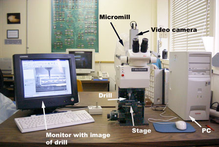
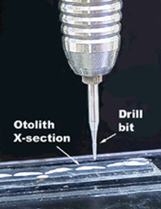
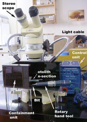
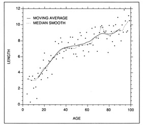
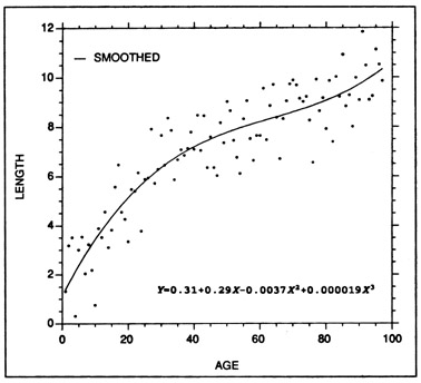
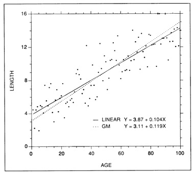
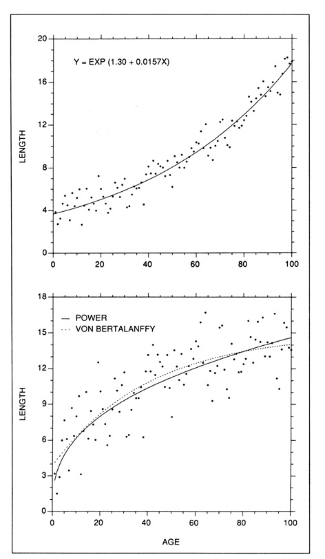
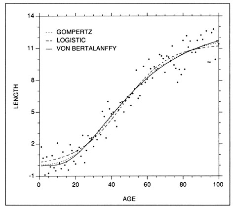
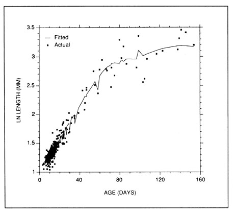
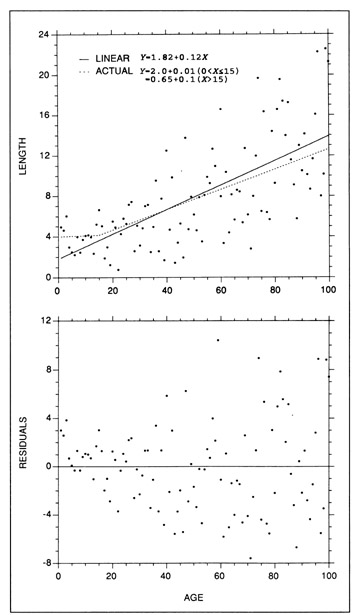
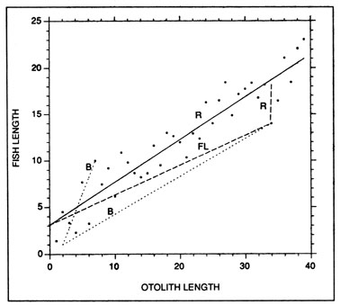
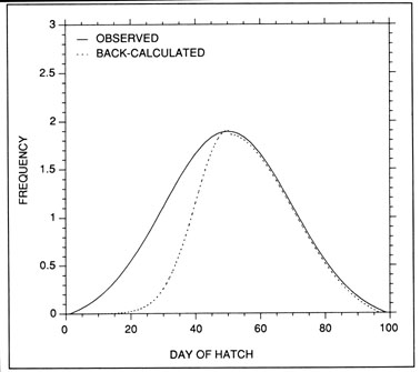
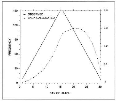
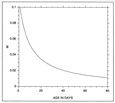
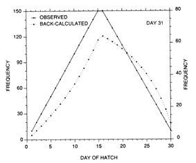
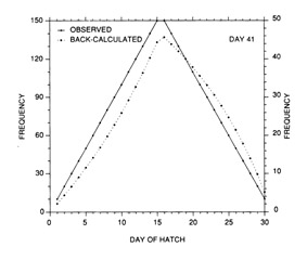
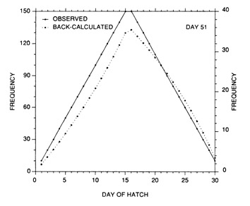
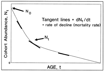
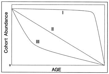
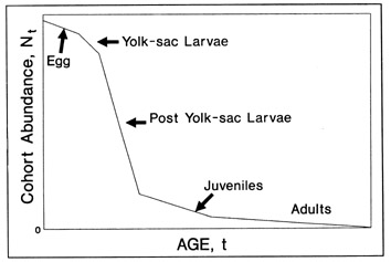
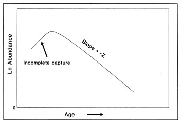
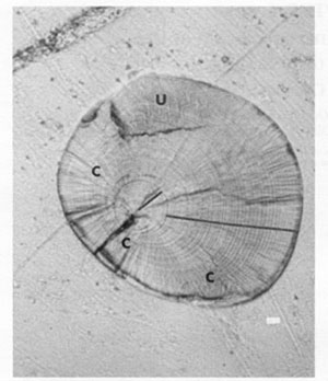
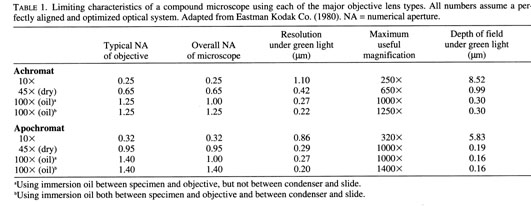
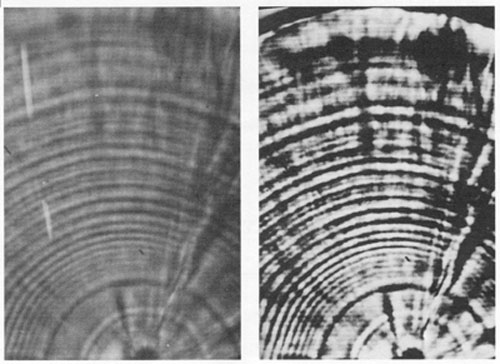
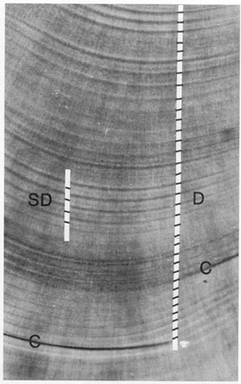
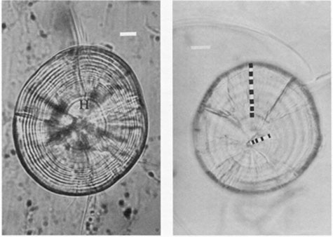
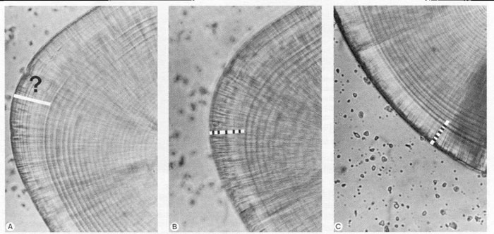
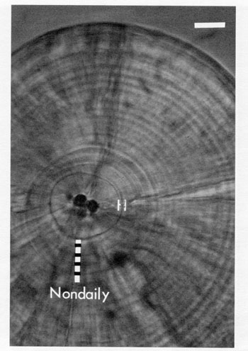
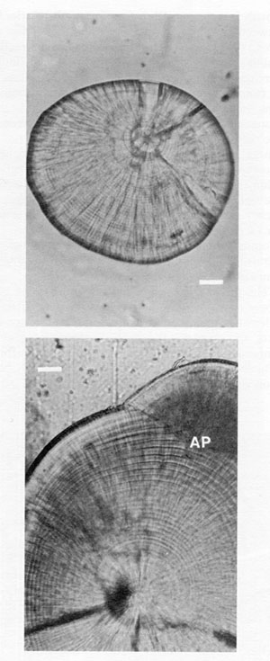
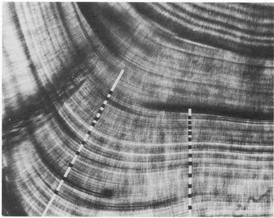
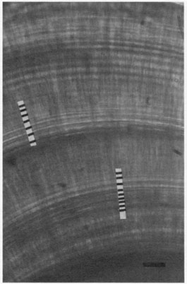
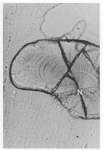
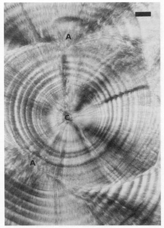